This is the first blog post of my life! I will be using this blog to post about anything that I want to share in statistics. For starter, I will run a linear regression with the iris dataset.
names(iris)## [1] "Sepal.Length" "Sepal.Width" "Petal.Length" "Petal.Width" "Species"Let’s predict Sepal.Length with Petal.Length and Petal.Width.
#separate into training and testing sets
set.seed(1234)
train_ind <- sample(nrow(iris), floor(0.8 * nrow(iris)))
iris_train <- iris[train_ind,]
iris_test <- iris[-train_ind,]

#run linear regression
iris_lm <- lm(Sepal.Length ~ Petal.Length + Petal.Width, data = iris_train)
summary(iris_lm)
##
## Call:
## lm(formula = Sepal.Length ~ Petal.Length + Petal.Width, data = iris_train)
##
## Residuals:
## Min 1Q Median 3Q Max
## -1.15417 -0.30771 -0.04347 0.29627 0.87021
##
## Coefficients:
## Estimate Std. Error t value Pr(>|t|)
## (Intercept) 4.11962 0.10794 38.164 < 2e-16 ***
## Petal.Length 0.57798 0.07426 7.783 3.11e-12 ***
## Petal.Width -0.39197 0.17184 -2.281 0.0244 *
## ---
## Signif. codes: 0 '***' 0.001 '**' 0.01 '*' 0.05 '.' 0.1 ' ' 1
##
## Residual standard error: 0.399 on 117 degrees of freedom
## Multiple R-squared: 0.7746, Adjusted R-squared: 0.7707
## F-statistic: 201 on 2 and 117 DF, p-value: < 2.2e-16The corresponding equation for iris_lm model is
\[\hat{y}_i = 4.12 + 0.58x_{1i} -0.39x_{2i}\]
Although all the coefficients show significance in terms of p-value, let’s create diagnostic plots to check if the model fits correctly.
par(mfrow = c(2, 2))
plot(iris_lm)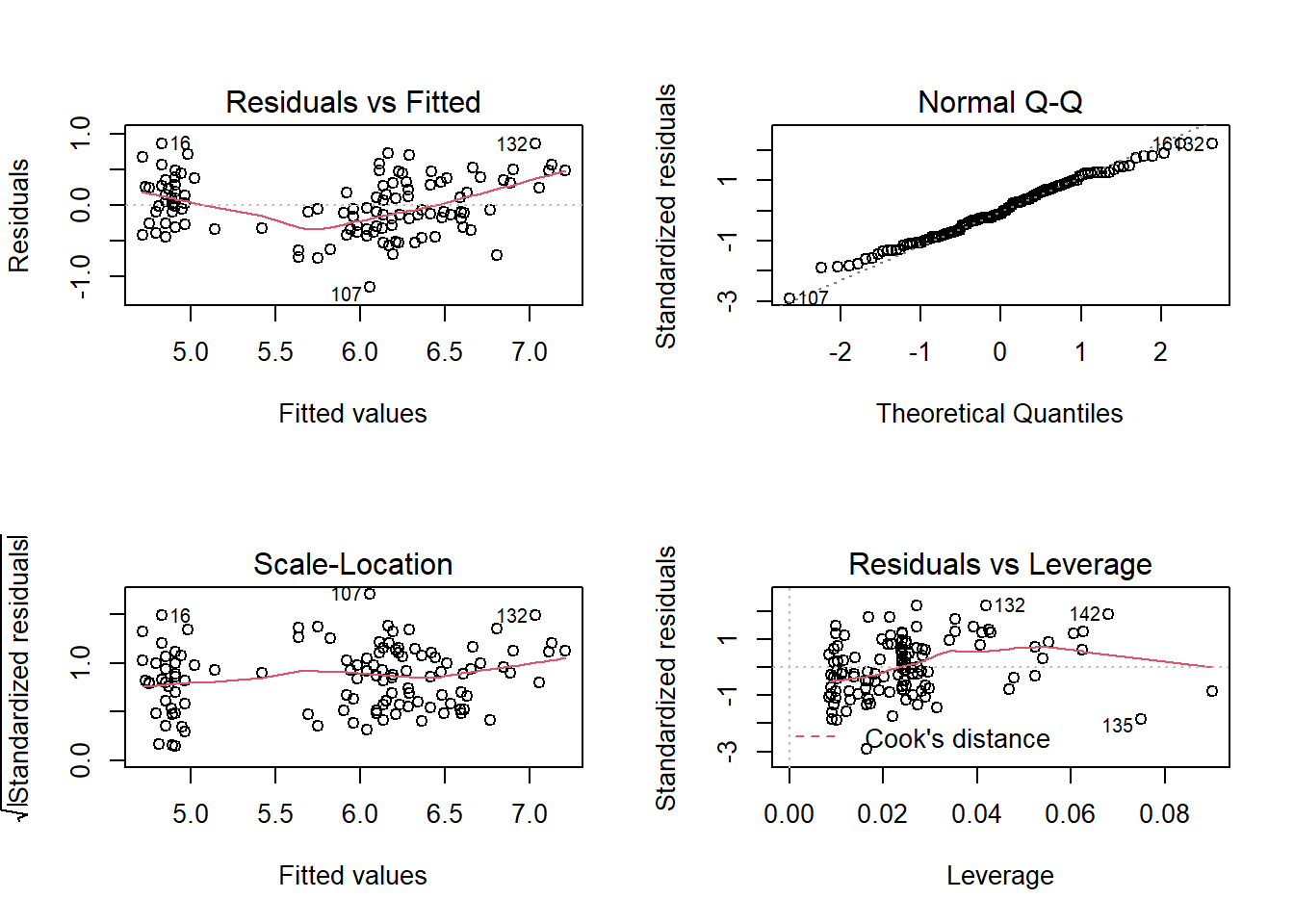
There seems to be a nonlinear trend in the Residuals vs Fitted diagnostic plot. This suggests that the true model may not be linear. As a result, I will include a quadratic term for the predictors.
The resulting quadratic model will take the form of \[\hat{y}_i = \hat{\beta}_0 + \hat{\beta}_{11}x_{1i} + \hat{\beta}_{12}x_{1i}^2 + \hat{\beta}_{21}x_{2i} + \hat{\beta}_{22}x_{2i}^2\]
iris_lm_quad <- lm(Sepal.Length ~ poly(Petal.Length, 2, raw = TRUE) + poly(Petal.Width, 2, raw = TRUE),
                   data = iris_train)
par(mfrow = c(2, 2))
plot(iris_lm_quad)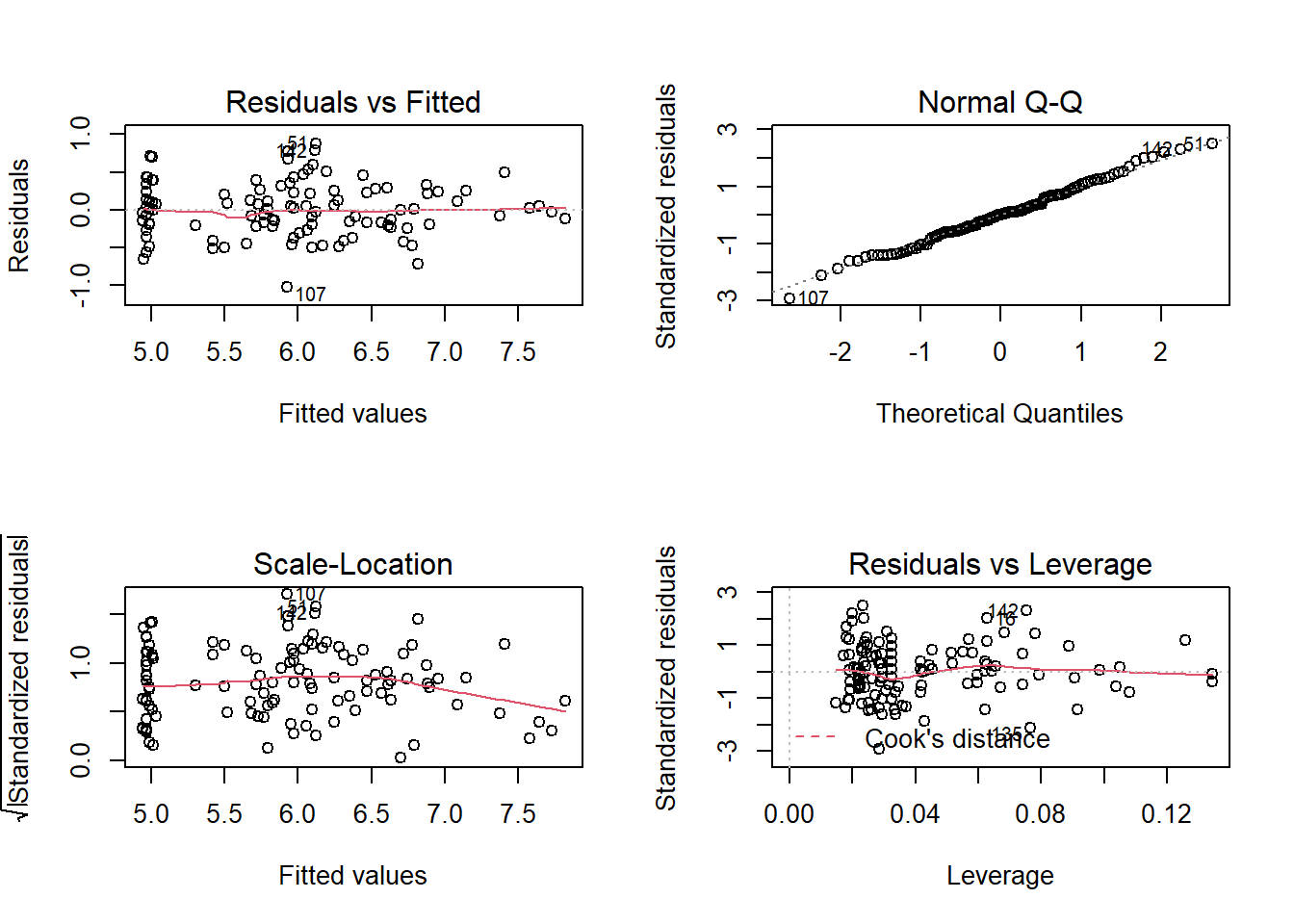
Now the non-linearity problem is gone! It looks as though there is an observation with leverage that is noticeably higher than that of others, but the observation has the Cook’s Distance well below 0.5; so I will not investigate further.
summary(iris_lm_quad)##
## Call:
## lm(formula = Sepal.Length ~ poly(Petal.Length, 2, raw = TRUE) +
## poly(Petal.Width, 2, raw = TRUE), data = iris_train)
##
## Residuals:
## Min 1Q Median 3Q Max
## -1.02406 -0.21390 0.00723 0.23591 0.87644
##
## Coefficients:
## Estimate Std. Error t value Pr(>|t|)
## (Intercept) 5.11499 0.25740 19.872 < 2e-16 ***
## poly(Petal.Length, 2, raw = TRUE)1 -0.29319 0.28206 -1.039 0.300764
## poly(Petal.Length, 2, raw = TRUE)2 0.10352 0.02726 3.797 0.000235 ***
## poly(Petal.Width, 2, raw = TRUE)1 0.31560 0.57731 0.547 0.585663
## poly(Petal.Width, 2, raw = TRUE)2 -0.17454 0.15563 -1.122 0.264380
## ---
## Signif. codes: 0 '***' 0.001 '**' 0.01 '*' 0.05 '.' 0.1 ' ' 1
##
## Residual standard error: 0.3555 on 115 degrees of freedom
## Multiple R-squared: 0.8241, Adjusted R-squared: 0.8179
## F-statistic: 134.7 on 4 and 115 DF, p-value: < 2.2e-16Judging from the summary, it is evident that the quadratic polynomial for Petal.Width is not very significant. Let’s remove that predictor and see how the model turns out.
iris_lm_quad <- update(iris_lm_quad, Sepal.Length ~ poly(Petal.Length, 2, raw = TRUE) + Petal.Width)
summary(iris_lm_quad)
##
## Call:
## lm(formula = Sepal.Length ~ poly(Petal.Length, 2, raw = TRUE) +
## Petal.Width, data = iris_train)
##
## Residuals:
## Min 1Q Median 3Q Max
## -0.99457 -0.22096 -0.00029 0.22785 0.87272
##
## Coefficients:
## Estimate Std. Error t value Pr(>|t|)
## (Intercept) 4.897726 0.169687 28.863 < 2e-16 ***
## poly(Petal.Length, 2, raw = TRUE)1 -0.009269 0.124526 -0.074 0.9408
## poly(Petal.Length, 2, raw = TRUE)2 0.077184 0.013859 5.569 1.68e-07 ***
## Petal.Width -0.308480 0.154025 -2.003 0.0475 *
## ---
## Signif. codes: 0 '***' 0.001 '**' 0.01 '*' 0.05 '.' 0.1 ' ' 1
##
## Residual standard error: 0.3559 on 116 degrees of freedom
## Multiple R-squared: 0.8221, Adjusted R-squared: 0.8175
## F-statistic: 178.7 on 3 and 116 DF, p-value: < 2.2e-16Now all the predictors are significant with the exception for the first order polynomial for Petal.Length. Nonetheless, I have to respect the hierarchy of higher order terms, so I’ll keep the coefficient.
The summary suggests that the model is statistically significant, and has the R-squared value of roughly 0.8. I’ll use this model to predict the Sepal.Length with the test dataset created in the beginning of this post.
y <- iris_test[,"Sepal.Length"]
y_hat <- predict(iris_lm_quad, iris_test[,c("Petal.Length", "Petal.Width")])

#calculate Root Mean Squared Error
rmse <- sqrt(sum((y - y_hat)^2)/length(y))
I used Root Mean Square Error to quantify the accuracy of the model, and it came out to be 0.379.
This marks the end of my first post. As I continue this blog, I hope to learn statistics and the models more in depth and become more adept at coming up with creative solutions for data analysis problems!