While I am reading Elements of Statistical Learning, I figured it would be a good idea to try to use the machine learning methods introduced in the book. I just finished a chapter on linear regression, and learned more about linear regression and the penalized methods (Ridge and Lasso). Since there is an abundant resource available online, it would be redundant to get into the details. I’ll quickly go over Ordinary Least Squares, Ridge, and Lasso regression, and quickly show an application of those methods in R.
Overview
All three of the models assume a linear model in which the output is a linear combination of the features (dependent variables).
\[y = \beta_0 + \Sigma_{i=1}^p\beta_ix_i\]
The difference comes from how the \(\beta_i\) are estimated.
Ordinary Least Squares method picks \(\hat{\beta}\) that minimizes the residual sum of squares: \[RSS(\beta) = \Sigma_{i=1}^N (y_i - (\hat{\beta}_0 + \Sigma_{i=1}^p\hat{\beta}_ix_i))^2\] Ridge Regression minimizes a function that takes into account RSS as well as the L2 Norm of \(\beta\) values: \[RSS_{ridge}(\beta) = \Sigma_{i=1}^N (y_i - (\hat{\beta}_0 + \Sigma_{i=1}^p\hat{\beta}_ix_i))^2 + \lambda\Sigma_{j=1}^p\beta_j^2\]
Lasso Regression is similar to ridge regression, except that it takes into account the L1 Norm of \(\beta\) values: \[RSS_{lasso}(\beta) = \Sigma_{i=1}^N (y_i - (\hat{\beta}_0 + \Sigma_{i=1}^p\hat{\beta}_ix_i))^2 + \lambda\Sigma_{j=1}^p|\beta_j|\]
\(\lambda\) is a hyperparameter that determines how much penalty to give to the norms. Higher \(\lambda\) will get the \(\beta\) reaching 0, while \(\lambda\) approaching 0 gets \(\beta\) close to the OLS estimates.
The extra penalty in the norms will cause the estimators to be “shrunk” in absolute values.
I wanted to try all three types of regression using R, so I grabbed a coffee rating dataset from tidy tuesday. I chose this dataset after skimming through a bunch in the list for its simple description and the availability of the numeric variables for a response variable as well as the feature variables.
The categorical variables could very well be coded into 1’s and 0’s for linear regression and the penalized regression, but the question remains: how can they also be standardized for “fair” evaluation? This is another topic in itself and I don’t plan to address this in this post, and only numerical variables will be included for the models.
Quick Data Clean
suppressPackageStartupMessages(library(tidyverse))## Warning: package 'ggplot2' was built under R version 4.0.5## Warning: package 'dplyr' was built under R version 4.0.5suppressPackageStartupMessages(library(naniar))
suppressPackageStartupMessages(library(gplots))
suppressPackageStartupMessages(library(glmnet))
# source of the data
# cofdat_tmp <-
# readr::read_csv('https://raw.githubusercontent.com/rfordatascience/tidytuesday/master/data/2020/2020-07-07/coffee_ratings.csv')
cofdat_tmp <-
readr::read_csv('coffee_ratings.csv')##
## -- Column specification --------------------------------------------------------
## cols(
## .default = col_character(),
## total_cup_points = col_double(),
## number_of_bags = col_double(),
## aroma = col_double(),
## flavor = col_double(),
## aftertaste = col_double(),
## acidity = col_double(),
## body = col_double(),
## balance = col_double(),
## uniformity = col_double(),
## clean_cup = col_double(),
## sweetness = col_double(),
## cupper_points = col_double(),
## moisture = col_double(),
## category_one_defects = col_double(),
## quakers = col_double(),
## category_two_defects = col_double(),
## altitude_low_meters = col_double(),
## altitude_high_meters = col_double(),
## altitude_mean_meters = col_double()
## )
## i Use `spec()` for the full column specifications.print(dim(cofdat_tmp))## [1] 1339 43print(head(cofdat_tmp))## # A tibble: 6 x 43
## total_cup_points species owner country_of_orig~ farm_name lot_number mill
## <dbl> <chr> <chr> <chr> <chr> <chr> <chr>
## 1 90.6 Arabica metad ~ Ethiopia "metad plc" NA meta~
## 2 89.9 Arabica metad ~ Ethiopia "metad plc" NA meta~
## 3 89.8 Arabica ground~ Guatemala "san marco~ NA NA
## 4 89 Arabica yidnek~ Ethiopia "yidnekach~ NA wole~
## 5 88.8 Arabica metad ~ Ethiopia "metad plc" NA meta~
## 6 88.8 Arabica ji-ae ~ Brazil NA NA NA
## # ... with 36 more variables: ico_number <chr>, company <chr>, altitude <chr>,
## # region <chr>, producer <chr>, number_of_bags <dbl>, bag_weight <chr>,
## # in_country_partner <chr>, harvest_year <chr>, grading_date <chr>,
## # owner_1 <chr>, variety <chr>, processing_method <chr>, aroma <dbl>,
## # flavor <dbl>, aftertaste <dbl>, acidity <dbl>, body <dbl>, balance <dbl>,
## # uniformity <dbl>, clean_cup <dbl>, sweetness <dbl>, cupper_points <dbl>,
## # moisture <dbl>, category_one_defects <dbl>, quakers <dbl>, color <chr>,
## # category_two_defects <dbl>, expiration <chr>, certification_body <chr>,
## # certification_address <chr>, certification_contact <chr>,
## # unit_of_measurement <chr>, altitude_low_meters <dbl>,
## # altitude_high_meters <dbl>, altitude_mean_meters <dbl># coffee type of score
ggplot(cofdat_tmp) +
geom_boxplot(aes(x = species, y = total_cup_points))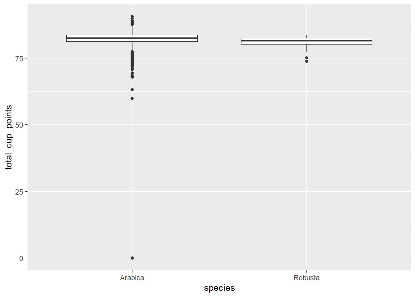
There’s one point where total rating is zero. It seems unusual for something to have a rating of complete 0, especially across all categories (except moisture?). I can’t imagine what it could have tasted like. In the end I’m not sure what led the judge to come to this conclusion, so for the time being, I removed this point as an outlier.
print(cofdat_tmp[cofdat_tmp$total_cup_points == 0,], width = Inf)## # A tibble: 1 x 43
## total_cup_points species owner country_of_origin farm_name
## <dbl> <chr> <chr> <chr> <chr>
## 1 0 Arabica bismarck castro Honduras los hicaques
## lot_number mill ico_number company altitude region
## <chr> <chr> <chr> <chr> <chr> <chr>
## 1 103 cigrah s.a de c.v. 13-111-053 cigrah s.a de c.v 1400 comayagua
## producer number_of_bags bag_weight in_country_partner
## <chr> <dbl> <chr> <chr>
## 1 Reinerio Zepeda 275 69 kg Instituto Hondureño del Café
## harvest_year grading_date owner_1 variety processing_method aroma
## <chr> <chr> <chr> <chr> <chr> <dbl>
## 1 2017 April 28th, 2017 Bismarck Castro Caturra NA 0
## flavor aftertaste acidity body balance uniformity clean_cup sweetness
## <dbl> <dbl> <dbl> <dbl> <dbl> <dbl> <dbl> <dbl>
## 1 0 0 0 0 0 0 0 0
## cupper_points moisture category_one_defects quakers color category_two_defects
## <dbl> <dbl> <dbl> <dbl> <chr> <dbl>
## 1 0 0.12 0 0 Green 2
## expiration certification_body
## <chr> <chr>
## 1 April 28th, 2018 Instituto Hondureño del Café
## certification_address
## <chr>
## 1 b4660a57e9f8cc613ae5b8f02bfce8634c763ab4
## certification_contact unit_of_measurement
## <chr> <chr>
## 1 7f521ca403540f81ec99daec7da19c2788393880 m
## altitude_low_meters altitude_high_meters altitude_mean_meters
## <dbl> <dbl> <dbl>
## 1 1400 1400 1400Since the data isn’t perfect, there are a lot of missing observations in some variables. naniar package has some tools that help with exploring the missingness of the data with clever visualizations. The first plot highlights the missing observations (row) for each variable (column). This can help with getting an idea of how much missingness there is and how the missingness is related across observations. Fortunately, the rating for each category are all present, so I will be able to keep all the observations. It seems like there is a fair amount of missing value in the altitude, so altitude will be omitted.
The plots after show more information about the missing observations.
# missing data explore
vis_miss(cofdat_tmp, sort_miss = TRUE)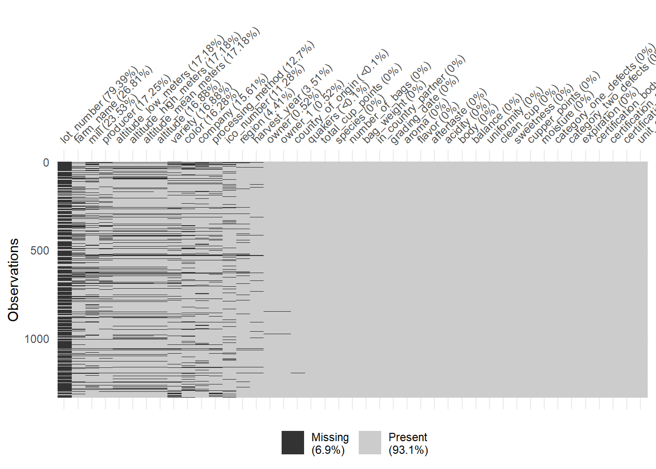
visdat::vis_dat(cofdat_tmp)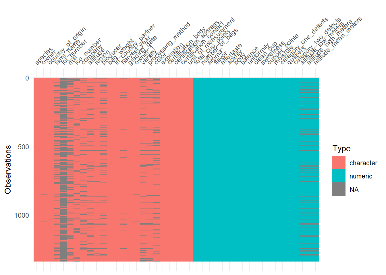
gg_miss_var(cofdat_tmp, show_pct = TRUE)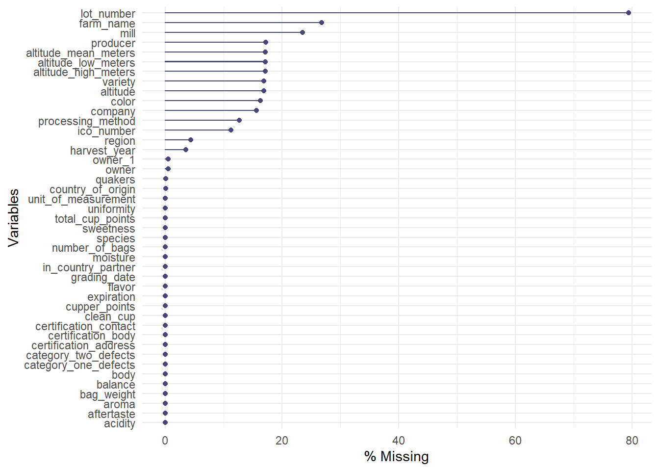
After applying my previous remarks, the data is prepared for analysis.
cofdat <- cofdat_tmp %>%
  filter(total_cup_points > 50) %>%
  select(
    total_cup_points, aroma, flavor, aftertaste, acidity,
    body, balance, uniformity, clean_cup, sweetness, cupper_points,
    moisture, category_one_defects, category_two_defects, quakers
  )
head(cofdat)
## # A tibble: 6 x 15
## total_cup_points aroma flavor aftertaste acidity body balance uniformity
## <dbl> <dbl> <dbl> <dbl> <dbl> <dbl> <dbl> <dbl>
## 1 90.6 8.67 8.83 8.67 8.75 8.5 8.42 10
## 2 89.9 8.75 8.67 8.5 8.58 8.42 8.42 10
## 3 89.8 8.42 8.5 8.42 8.42 8.33 8.42 10
## 4 89 8.17 8.58 8.42 8.42 8.5 8.25 10
## 5 88.8 8.25 8.5 8.25 8.5 8.42 8.33 10
## 6 88.8 8.58 8.42 8.42 8.5 8.25 8.33 10
## # ... with 7 more variables: clean_cup <dbl>, sweetness <dbl>,
## # cupper_points <dbl>, moisture <dbl>, category_one_defects <dbl>,
## # category_two_defects <dbl>, quakers <dbl>There is one missing observation in quaker variable, which stores the number of “bad” beans mixed in with the good beans. This is removed as well.
# one missing value in quakers variable
cofdat %>% miss_var_summary()
## # A tibble: 15 x 3
## variable n_miss pct_miss
## <chr> <int> <dbl>
## 1 quakers 1 0.0747
## 2 total_cup_points 0 0
## 3 aroma 0 0
## 4 flavor 0 0
## 5 aftertaste 0 0
## 6 acidity 0 0
## 7 body 0 0
## 8 balance 0 0
## 9 uniformity 0 0
## 10 clean_cup 0 0
## 11 sweetness 0 0
## 12 cupper_points 0 0
## 13 moisture 0 0
## 14 category_one_defects 0 0
## 15 category_two_defects 0 0cofdat <- na.omit(cofdat)I can plot box plots and histogram to skim through the distribution of each variables.
cof_long <- cofdat %>% pivot_longer(cols = everything(), names_to = "Var", values_to = "value")

ggplot(cof_long) +
  geom_boxplot(aes(x = Var, y = value)) +
  theme(axis.text.x = element_text(angle = 90, hjust = 1, vjust = 0.3, size = 8), axis.title = element_blank())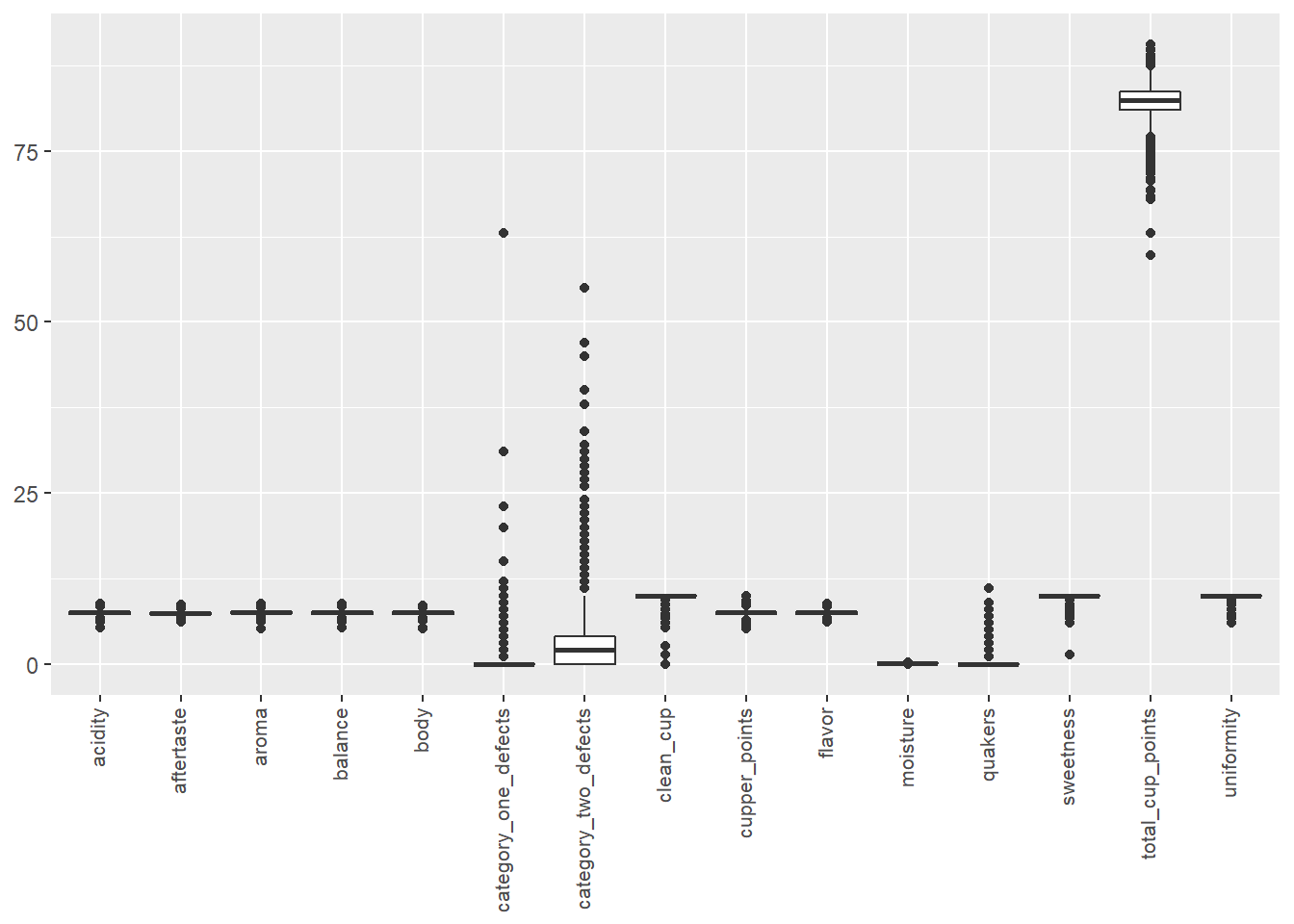
ggplot(cof_long) +
  geom_histogram(aes(value), bins = 50) +
  facet_wrap(facets = ~Var, scales = "free")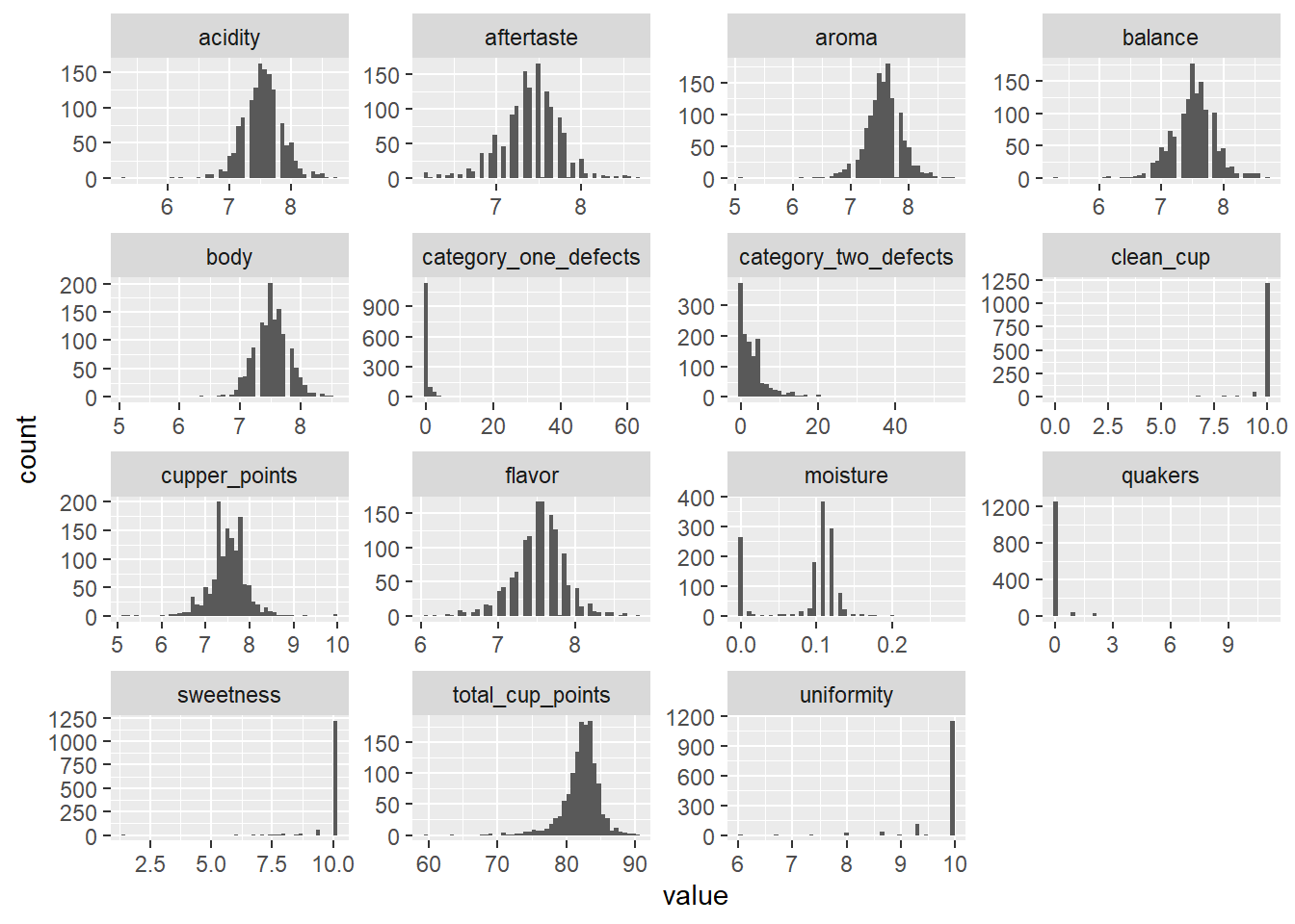
One notable thing is that category_one_defects, category_two_defects, and quakers comparatively have a lot of 0’s than non-zero values. These variables look like an indicator of defects, so they should negatively affect the total score. I am curious to see how they will affecting the score.
Lastly, I checked the correlation between all the variables included in the model. Ideally, I would not want to have a high correlation among the variables since that could lead to the inflation of the standard error for \(\beta\) estimates, possibly making the \(\beta\) very unstable.
cof_cor <- cor(cofdat)

heatmap.2(cof_cor, symm = TRUE, col = bluered(100), trace = "none", main = "Correlation Between Variables\n(with Hierarchical Clustering)")
As I suspected, I see some strong correlations among the ratings. It does make sense to see this since a good bean is bound to have multiple positive characteristics. At the top of the heatmap we have flavor and aftertaste. If a food has good flavor, I would expect to have a pleasant aftertaste. Another interesting takeaway from the heatmap is how the three of last four variables,
 category_one_defects, category_two_defects, and quakers, which are indicators of poor quality, are clustered out of the other ratings. Frankly, I don’t know why moisture joined the party there because I have no knowledge of coffee bean ratings. The association looks very weak, so it could be a random chance. But it could very well be that higher rating for moisture is a bad thing.
In the end, I decided to keep all the variables for regression since all of these variables were likely to have been considered for the final score.
Running the Models
Linear Regression with Ordinary Least Squares
This part is simple, as I only need to use lm() and summary() to review the output.
linreg <- lm(total_cup_points ~ ., data = cofdat)
summary(linreg)
##
## Call:
## lm(formula = total_cup_points ~ ., data = cofdat)
##
## Residuals:
## Min 1Q Median 3Q Max
## -0.42978 -0.00374 -0.00085 0.00751 0.10215
##
## Coefficients:
## Estimate Std. Error t value Pr(>|t|)
## (Intercept) 1.289e-02 1.561e-02 0.826 0.409
## aroma 9.992e-01 2.032e-03 491.712 < 2e-16 ***
## flavor 9.993e-01 2.880e-03 346.939 < 2e-16 ***
## aftertaste 1.000e+00 2.633e-03 379.855 < 2e-16 ***
## acidity 9.973e-01 2.086e-03 478.222 < 2e-16 ***
## body 1.002e+00 1.962e-03 510.931 < 2e-16 ***
## balance 1.002e+00 2.006e-03 499.669 < 2e-16 ***
## uniformity 1.002e+00 9.923e-04 1009.913 < 2e-16 ***
## clean_cup 9.997e-01 7.039e-04 1420.342 < 2e-16 ***
## sweetness 9.982e-01 8.372e-04 1192.313 < 2e-16 ***
## cupper_points 9.981e-01 1.557e-03 641.145 < 2e-16 ***
## moisture 8.139e-03 9.066e-03 0.898 0.370
## category_one_defects -1.681e-03 1.746e-04 -9.631 < 2e-16 ***
## category_two_defects -3.473e-04 8.653e-05 -4.013 6.32e-05 ***
## quakers -2.325e-04 5.058e-04 -0.460 0.646
## ---
## Signif. codes: 0 '***' 0.001 '**' 0.01 '*' 0.05 '.' 0.1 ' ' 1
##
## Residual standard error: 0.01534 on 1322 degrees of freedom
## Multiple R-squared: 1, Adjusted R-squared: 1
## F-statistic: 2.929e+06 on 14 and 1322 DF, p-value: < 2.2e-16Ridge Regression
I use the package glmnet to use ridge and lasso methods. The elastic net penalty in glmnet is given by:
\[\frac{(1-\alpha)}{2}||\beta_j||_2^2+\alpha||\beta_j||_2\]
Whether the regression is ridge, lasso, or in between is controlled by \(\alpha\), with \(\alpha = 1\) being lasso and \(\alpha = 0\) being ridge.
To determine the most appropriate \(\lambda\), cross validation can be used. cv.glmnet does the heavy lifting for me and calculates the MSE for each lambda after doing cross validation. I opt for the highest \(\lambda\) whose MSE is within 1 sd of the lowest MSE across all the \(\lambda\)s. I believe this leads to better generalization while maintaining low training error.
This short code will run cross-validation with various \(\lambda\)s, choose the appropriate lambda, and get a final model with that lambda.
# Choose the value of lambdas I'd like to test
lambdas <- exp(1)^seq(3, -10, by = -0.05)

# Cross validation with different lambdas
ridge <- cv.glmnet(
    x = as.matrix(cofdat[, -1]),
    y = cofdat$total_cup_points,
    alpha = 0,
    standardize = TRUE, # standardizes training data
    lambda = lambdas
  )

# choose lambda.1se
print(ridge$lambda.1se)
## [1] 0.03877421ridge_final <- glmnet(
x = as.matrix(cofdat[, -1]),
y = cofdat$total_cup_points,
alpha = 0,
standardize = TRUE, # standardizes training data
lambda = ridge$lambda.1se
)
print(ridge_final$a0)## s0
## 0.3755191print(ridge_final$beta)## 14 x 1 sparse Matrix of class "dgCMatrix"
## s0
## aroma 0.9907920628
## flavor 1.0214067393
## aftertaste 1.0011881996
## acidity 0.9888159329
## body 0.9939766384
## balance 1.0014300201
## uniformity 0.9975419726
## clean_cup 0.9884834152
## sweetness 0.9890917946
## cupper_points 0.9856624624
## moisture 0.0051675667
## category_one_defects -0.0022493552
## category_two_defects -0.0008581067
## quakers 0.0001926588Just a couple things to note here:
xexpects a matrix input where each column is a feature and each row is an observation. The data cleaning step is usually conveniently done with adata.framebut ifdata.frameis passed intox, then an error will be put out.standardizedoes the scaling (standardization) of the feature inputs for me and returns the rescaled-version of the coefficients. If you have already done the standardization yourself, then you can setstandardizeto FALSE.
LASSO
lasso <- cv.glmnet(
  x = as.matrix(cofdat[, -1]),
  y = cofdat$total_cup_points,
  alpha = 1,
  standardize = TRUE, # standardizes training data
  lambda = lambdas
)

# choose lambda.1se
print(lasso$lambda.1se)
## [1] 0.009095277lasso_final <- glmnet(
x = as.matrix(cofdat[, -1]),
y = cofdat$total_cup_points,
alpha = 1,
standardize = TRUE, # standardizes training data
lambda = lasso$lambda.1se
)
print(lasso_final$a0)## s0
## 0.486362print(lasso_final$beta)## 14 x 1 sparse Matrix of class "dgCMatrix"
## s0
## aroma 0.9884542
## flavor 1.0168211
## aftertaste 1.0030134
## acidity 0.9852781
## body 0.9839906
## balance 1.0016683
## uniformity 0.9935998
## clean_cup 0.9951121
## sweetness 0.9875308
## cupper_points 0.9874171
## moisture .
## category_one_defects .
## category_two_defects .
## quakers .Results
Let’s see the results and see how the coefficients differ.
coefs <- data.frame(variable = colnames(cofdat)[-1])
coefs$lm <- linreg$coefficients[coefs$variable]
coefs$ridge <- ridge_final$beta[coefs$variable,]
coefs$lasso <- lasso_final$beta[coefs$variable,]
coefs_long <- coefs %>%
mutate(variable = factor(variable, sort(variable))) %>%
pivot_longer(cols = c("lm", "ridge", "lasso"), names_to = "Method", values_to = "Coefficients") %>%
filter(abs(Coefficients) > 0) %>%
mutate(Method = factor(Method, c("lm", "ridge", "lasso"), labels = c("Linear Regression", "Ridge", "Lasso")))
coefs_long$low <- ifelse(coefs_long$Coefficients < 0.1, TRUE, FALSE)
ggplot(filter(coefs_long)) +
facet_grid(rows = vars(low), scales = "free_y") +
geom_point(aes(x = variable, y = Coefficients, color = Method)) +
ggtitle("Coefficient Comparison across Three Models") +
theme(axis.text.x = element_text(angle = 45, vjust = 1, hjust = 1))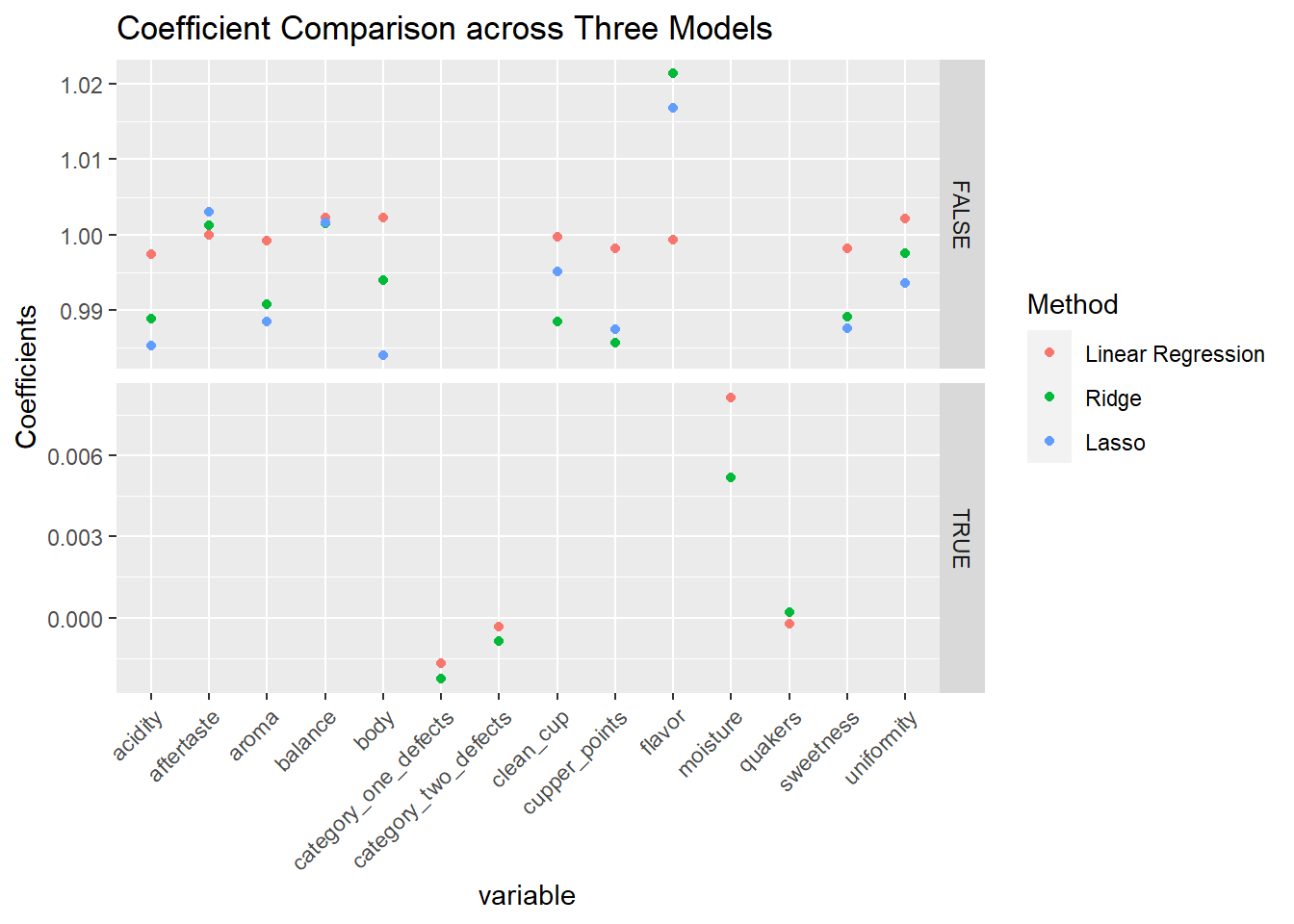 You can see that the coefficients are all around zero, with the exception of the four variables that indicate poor quality. I think it should come clear from this result that the final rating,
 total_cup_points, is actually a simple sum of those ratings! Honestly, I hadn’t thought this through when I was choosing the dataset and running the regressions. I should have seen this beforehand in hindsight; there are 10 rating features, all ranging from 0 to 10, and the total score is on a range from 0 to 100.
You can still see the shrinkage effect in the penalized regression in the coefficient comparison plot above. Ridge and Lasso’s coefficients are lower in absolute value than the OLS methods for the most part. Furthermore, the coefficients for category_one_defects, category_two_defects, moisture, and quakers are all shrunk to 0 for Lasso. All the methods seem to capture the relationship between the 10 rating features and the final score.
There are some cases where the final score is not exactly a total sum of the 10 variables, and this makes the coefficients to deviate slightly from 1.
Ending Remark
In this post, I grabbed a coffee dataset to practice penalized regression and see the shrinkage effect in action. We observed some of the variables being shrunk to zero as the penalty increases in Lasso. We were able to see that with the help of the regression models that the final score is simply a linear combination of 10 different ratings for characteristics for coffee beans. Unfortunately, it was difficult to see if the extra generalization from the penalized methods helped with prediction of the response due to the nature of the variables. When the time comes, I will try these methods on a different datasets and see if the generalizations help with making a better model.