LDA, Linear Discriminant Analysis, is a classification method and a dimension reducion technique. I’ll focus more on classification. LDA calculates a linear discriminant function (which arises from assuming Gaussian distribution) for each class, and chooses a class that maximizes such function. The linear discriminant function therefore dictates a linear decision boundary for choosing a class. The decision boundary should be linear in the feature space. Discriminant analysis itself isn’t inherently linear. LDA is just a special case of discriminant analysis that arises from the assumption that all the classes share the same covariance matrix.
Discriminant function of class \(k\): \[\delta(x) = x^T \Sigma^{-1}\mu_k-\frac{1}{2}\mu_k^T\Sigma^{-1}\mu_k + log(\pi_k)\] where
\(\mu_k\) = mean for class k
\(\Sigma\) = pooled sample mean
\(\pi_k\) = prior for class k.
Usually these parameters are unkown, and they are derived from the sample.
To predict the class for new data points, calculate the discriminant function for each class
Again, this result arises with the assumptions that:
- each class is from a normal distribution with class-specific mean \((\mu_k)\)
- the normal distributions share a common variance \((\Sigma)\)
Example with a 2-class case.
First, create training samples & test samples
library(tidyverse)
library(mixtools)
library(MASS)
library(latex2exp)
library(kableExtra)
library(knitr)
library(formattable)

set.seed(285)
S <- matrix(c(1,0.5,0.5,1), 2); n_each <- 50 # set equal covariance for all
true_mu_a <- c(1,1); true_mu_b <- c(3,3)

#training samples
a <- mvrnorm(n_each, mu = true_mu_a, Sigma = S) # bivariate normal distribution with mean = (1,1)
b <- mvrnorm(n_each, mu = true_mu_b, Sigma = S) # bivariate normal distribution with mean = (3,3)
mydf <- data.frame(x1 = c(a[,1], b[,1]), x2 = c(a[,2], b[,2]), cl = rep(c('A','B'),each = n_each))
print(head(mydf))
## x1 x2 cl
## 1 1.2884039 1.695735 A
## 2 0.6343596 1.303904 A
## 3 3.0019974 1.067433 A
## 4 -1.4700693 -1.066326 A
## 5 1.0066906 1.972617 A
## 6 1.3897566 1.871020 A#create test points
test_n_each <- 40
a_test <- mvrnorm(test_n_each, mu = true_mu_a, Sigma = S)
b_test <- mvrnorm(test_n_each, mu = true_mu_b, Sigma = S)
mytest <- data.frame("x1" = c(a_test[,1], b_test[,1]), "x2" = c(a_test[,2], b_test[,2]))
true_class <- rep(c("A", "B"), each = test_n_each)Distribution of the data:
plot(mydf[,1], mydf[,2], col = factor(mydf[,3]), pch = 1, main = "Data distribution", xlab = "x1", ylab = "x2")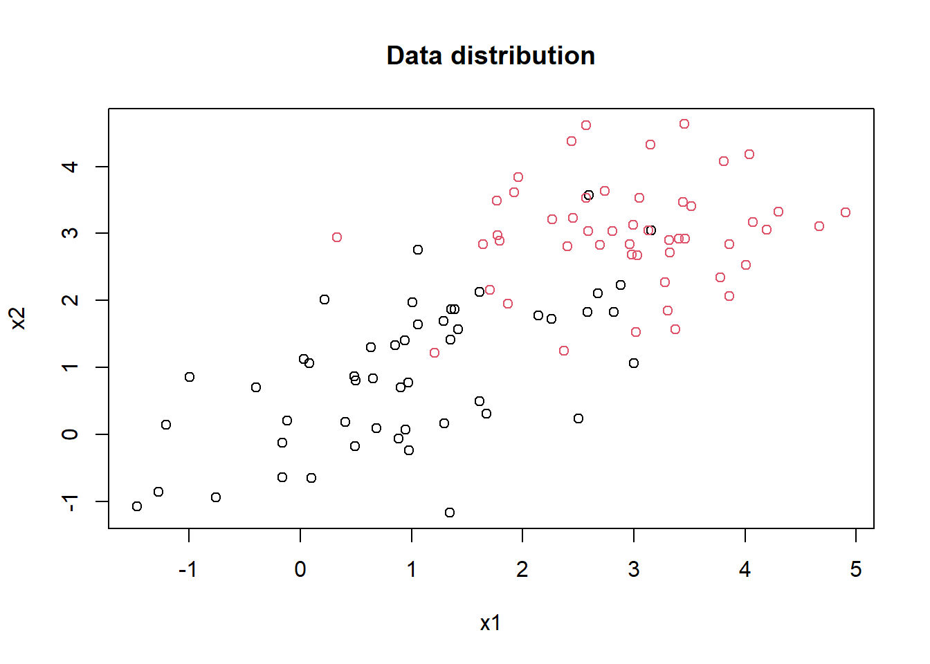
Assuming that we don’t know the true \(\mu\) and \(\Sigma\), estimate them with the sample mean and sample covariance matrix.
mu1 <- apply(mydf[mydf$cl == "A",c(1,2)], 2, mean) # sample mean for class A
mu2 <- apply(mydf[mydf$cl == "B", c(1,2)], 2, mean) # sample mean for class B
centered <- as.matrix(
  mydf[,c(1,2)] - rbind(matrix(rep(mu1, n_each), ncol = 2, byrow = TRUE),
                        matrix(rep(mu2, n_each), ncol = 2, byrow = TRUE)))
varcov <- t(centered) %*% centered / (nrow(centered) - 2) # pooled variace-covariance matrix
varcov_inv <- solve(varcov)| \(\hat{\mu}_A\) | \(\hat{\mu}_B\) | |
|---|---|---|
| x1 | 0.9654044 | 2.951309 |
| x2 | 0.9193072 | 2.998684 |
| x1 | x2 | |
|---|---|---|
| x1 | 1.1477071 | -0.5516819 |
| x2 | -0.5516819 | 1.3686371 |
The following functions use the discriminant function to calculate the scores.
#used to calculate the discriminant functions
calc_score <- function(x, mu, varcov_inv, prop){
  as.numeric((x %*% varcov_inv %*% mu) - 0.5 * (mu %*% varcov_inv %*%  mu) + log(prop))
}
calc_score_A <- function(x){
  calc_score(x, mu1, varcov_inv, 0.5)
}
calc_score_B <- function(x){
  calc_score(x, mu2, varcov_inv, 0.5)
}
Now that I have the sample mean, sample covariance matrix, and a way to calculate and compare the scores, I can make predictions.
test_scores <- data.frame("A_score" = apply(mytest, MARGIN = 1, calc_score_A),
                          "B_score" = apply(mytest, MARGIN = 1, calc_score_B)) %>%
  mutate("Prediction" = ifelse(A_score > B_score, "A", "B"))
test_scores %>%
        mutate(
          A_score = ifelse(
            A_score > B_score,
            cell_spec(round(A_score, 4), format = "html", bold = TRUE),
            round(A_score, 4)),
          B_score = ifelse(
            B_score > A_score,
            cell_spec(round(B_score, 4), format = "html", bold = TRUE),
            round(B_score, 4)
          )
        ) %>%
  kable('html', escape = FALSE) %>%
  kable_styling(full_width = FALSE) %>%
scroll_box(height = "300px")| A_score | B_score | Prediction |
|---|---|---|
| -0.1759 | -3.278 | A |
| -0.3776 | -4.0634 | A |
| -0.107 | -3.0551 | A |
| 0.4823 | -1.1914 | A |
| -0.5195 | -4.2361 | A |
| -1.3337 | -7.0005 | A |
| 1.1516 | 0.9352 | A |
| 1.0608 | 0.6911 | A |
| -1.6188 | -7.8291 | A |
| -1.5134 | -7.6937 | A |
| 0.5681 | -1.2204 | A |
| 0.0126 | -2.6787 | A |
| 0.5729 | -0.9481 | A |
| -0.3874 | -3.5652 | A |
| -0.4229 | -4.3903 | A |
| 0.3493 | -1.5217 | A |
| 1.7273 | 2.5746 | B |
| -1.0234 | -6.0853 | A |
| -1.9975 | -9.0358 | A |
| -0.2693 | -3.9278 | A |
| 0.8209 | -0.5283 | A |
| 0.3686 | -1.6875 | A |
| 2.367 | 4.8856 | B |
| -1.3572 | -7.0641 | A |
| -0.734 | -5.1947 | A |
| -0.2281 | -3.74 | A |
| 0.3025 | -1.7457 | A |
| -0.1377 | -3.3154 | A |
| 0.154 | -2.0848 | A |
| 0.6786 | -0.4303 | A |
| 0.4324 | -1.6249 | A |
| 0.4964 | -1.2815 | A |
| -2.5051 | -10.7099 | A |
| 0.6792 | -0.3356 | A |
| -0.3274 | -3.7487 | A |
| -0.5677 | -4.8283 | A |
| -0.2977 | -3.5145 | A |
| -0.2623 | -3.7453 | A |
| -0.0615 | -3.0913 | A |
| 1.8722 | 3.2393 | B |
| 3.4055 | 8.0866 | B |
| 4.3429 | 11.0935 | B |
| 1.922 | 3.1492 | B |
| 3.4832 | 8.5813 | B |
| 3.0456 | 6.7597 | B |
| 3.0459 | 6.9929 | B |
| 3.1109 | 7.3301 | B |
| 1.9522 | 3.3569 | B |
| 2.4712 | 5.2453 | B |
| 1.1155 | 0.6139 | A |
| 1.6235 | 2.4427 | B |
| 3.8512 | 9.3066 | B |
| 4.3328 | 10.9274 | B |
| 0.5177 | -1.3228 | A |
| 1.9686 | 3.2308 | B |
| 1.8329 | 3.0792 | B |
| 0.7742 | -0.1188 | A |
| 2.9128 | 6.5723 | B |
| 1.5093 | 1.7485 | B |
| 2.3112 | 4.6208 | B |
| 1.8433 | 3.0966 | B |
| 2.605 | 5.5216 | B |
| 2.1003 | 3.7596 | B |
| 1.2751 | 1.1232 | A |
| 1.8186 | 3.0485 | B |
| 2.9834 | 6.5644 | B |
| 4.964 | 12.9167 | B |
| 2.7923 | 6.0654 | B |
| 1.9884 | 3.6019 | B |
| 0.7061 | -0.82 | A |
| 2.7743 | 6.0155 | B |
| 1.8871 | 3.5962 | B |
| 1.4034 | 1.6698 | B |
| 4.9516 | 12.9317 | B |
| 1.3665 | 1.4068 | B |
| 4.2016 | 10.6066 | B |
| 1.5156 | 2.0366 | B |
| 2.8598 | 6.2117 | B |
| 2.535 | 5.3056 | B |
| 3.6067 | 8.3908 | B |
You can see that the classification is based on whichever score is higher
Compare the results with R’s built in LDA function.
myLDA <- lda(cl ~ ., data = mydf) # built in LDA
mypred <- predict(myLDA, mytest)

all(test_scores$Prediction == mypred$class)
## [1] TRUEI’m interested in seeing what the decision boundary looks like. It’s simple. Since the classification is based on discriminant function, I just have to find out for which values of x1 and x2 the scores for both classes are equal.
i.e.
\(\delta_A(x) - \delta_B(x) = x^T \Sigma^{-1}\mu_A-\frac{1}{2}\mu_A^T\Sigma^{-1}\mu_A + log(\pi_A) - x^T \Sigma^{-1}\mu_B+\frac{1}{2}\mu_B^T\Sigma^{-1}\mu_B - log(\pi_B) \\ = x^T\Sigma^{-1}(\mu_A-\mu_B) + \big(-\frac{1}{2}\mu_A^T\Sigma^{-1}\mu_A+\frac{1}{2}\mu_B^T\Sigma^{-1}\mu_B\big)\)
coeff_tmp <- varcov_inv %*% (mu1 - mu2)
intercept_tmp <- - 0.5 * (mu1 %*% varcov_inv %*% mu1) + 0.5 * (mu2 %*% varcov_inv %*% mu2)

slope <- coeff_tmp[1] / -coeff_tmp[2]
intercept <- intercept_tmp / -coeff_tmp[2]

message(paste0("slope: ", slope, ", intercept: ", intercept))
## slope: -0.646784109561366, intercept: 3.22562929419369plot(mydf[,1], mydf[,2], col = factor(mydf[,3]), pch = 1, main = "Linear Boundary with Training Points", xlab = "x1", ylab = "x2")
abline(b = slope, a = intercept)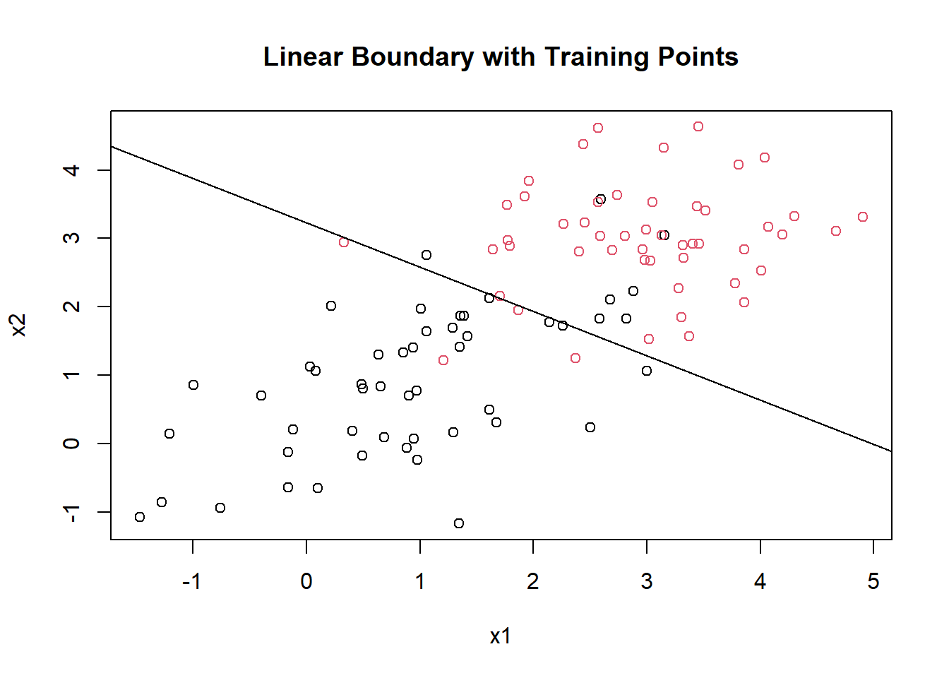
plot(mytest[,1], mytest[,2], col = factor(test_scores[,3]), pch = 1, main = "Linear Boundary with Test Points", xlab = "x1", ylab = "x2")
abline(b = slope, a = intercept)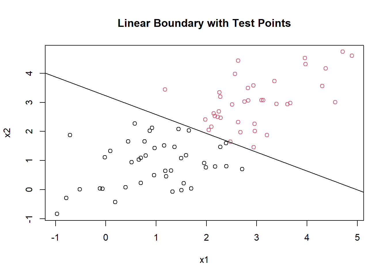
The line doesn’t perfectly separate the training data points because they are not linearly separable without any transformation. But you can see that the class predictions are based on which side of the line the points lie on.
An interesting thing to point out is the relation between LDA and linear discriminant analysis. If I set each class as 1 and -1 (A and B resp.), run linear regression with the intercept, and classify based on size relative to 0, the predictions are the same!
mydf <- mydf %>% mutate(y = ifelse(cl == "A", 1, -1))

mylm <- lm(y ~ x1 + x2, mydf)
classes <- ifelse(predict(mylm, mytest) > 0, "A", "B")
all(classes == test_scores$Prediction)
## [1] TRUEI’ve wanted to try implementing my own vanilla version of the LDA, and visualize the results. It definitely helps understanding the problem in a simple case (like running LDA in the two dimensional case), and then generalize the results to a more complex case.