In my first machine learning class, in order to learn about the theory behind PCA (Principal Component Analysis), we had to learn about variance-covariance matrix. I was concurrently taking a basic theoretical probability and statistics, so even the idea of variance was still vague to me. Despite the repeated attempts to understand covariance, I still had trouble fully capturing the intuition behind the covariance between two random variables. Even now, application and verification of correct usage of mathematical properties of covariance requires intensive googling. I want to use this post to review covariance and its properties.
Basic Idea : Covariance of two random variables \(X\) and \(Y\), also written as \(cov[X,Y]\) and \(\sigma_{XY}\), is a strength of linear relationship between two random variables. It can be used to determine the directional strength of relationship between two random variables. Covariance is easily visualized by observing a distribution of bivariate normal distribution.
Consider a bivariate normal distribution (non degenerate) with random variables X and Y, where \(\mu_X, \mu_Y = 0\), \(\sigma_X, \sigma_Y = 1\), and \(\sigma_{XY}\) takes different values.
library(MASS)
library(mixtools)
## Warning: package 'mixtools' was built under R version 4.0.5## mixtools package, version 1.2.0, Released 2020-02-05
## This package is based upon work supported by the National Science Foundation under Grant No. SES-0518772.set.seed(1234)
gen_binormplot <- function(N, mu_vec, Sigma, ...){ #function that creates a plot for randomly generated bivariate normal distribution
biv_norm <- mvrnorm(
n = N,
mu = mu_vec,
Sigma = Sigma
)
plot(x = biv_norm[, 1],
y = biv_norm[, 2],
main = bquote('bivariate normal distribution when' ~ sigma['xy'] == .(Sigma[2])),
xlab = 'x',
ylab = 'y',
col = 'dark grey',
...)
for (ellipse_alpha in seq(0, 1, 0.2)){
ellipse(mu_vec,
Sigma,
alpha = ellipse_alpha,
type = 'l',
col = 'red',
lwd = 1.5)
}
}
N <- 1000
mu_x <- 0; mu_y <- 0
var_x <- 1; var_y <- 1
cov_xy <- c(-0.9, 0.9, -0.7, 0.7, -0.3, 0.3, 0)
par(mfrow = c(2,2), mai = c(0.5, 0.5, 0.5, 0.5))
for (plt in 1:length(cov_xy)){
Sig <- matrix(c(var_x, cov_xy[plt], cov_xy[plt], var_y), nrow = 2, byrow = TRUE)
gen_binormplot(N, c(mu_x, mu_y), Sig, xlim = c(-3, 3), ylim = c(-3, 3))
}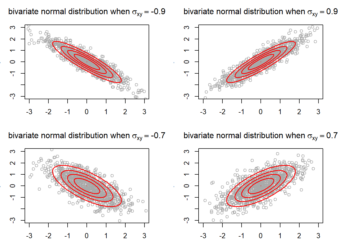
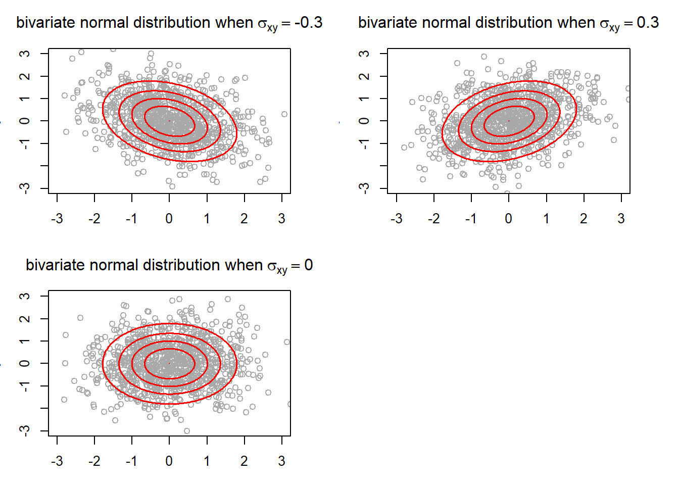 The ellipses show the region in which a certain portion of the points from a bivariate normal distribution falls into. The outermost ellipse contains 95% of the points. Also, the ellipses allows us to see more easily the general trend that the two random variables have. As you can see, negative covariance is associated with inverse relationship between X and Y, and positive covariance is associated with direct relationship. Furthermore, the ellipses tend to get wider as the absolute value of covariance decreases. This is because lower absoluate value of covariance is regarded as the two random variables having a “weaker” relationship. In fact, the ellipses in the case where \(\sigma_{XY} = 0\) would be a perfect circle had the plot size been square (which is also ascribed to the variance of X and Y being equal).
Mathematical Definition: \(Cov[X, Y] = E\big[(X-E[X])(Y-E[Y])\big]\)
In words, the covariance of random variables \(X\) and \(Y\) is an expectation of the product of the two variables’ deviation from the mean.
From this definition, I like to understand the previously seen trend (where negative covariance is related to inverse relationship and positive covariance is related to direct relationship) by thinking of extreme cases. If X and Y were to have inverse (linear) relationship, where increasing X is related to decreasing Y, then higher values of X, which is above its mean will be paired with lower values of Y, which is below the mean. Then the deviation for X and Y will have opposite signs. So the expected value of their product would be negative. Similar reason applies for positive covariance.
Covariance can also be written as: \(Cov[X, Y] = E[XY] - E[X]E[Y]\).
With this formula, it is easier to see why two independent random variables have covariance of 0, since for two independent random variables X and Y, \(E[XY] = E[X]E[Y]\). However, the converse is not always true.
A simple example:
\(X \sim unif(-1, 1)\)
\(Y = X^2\)
Then \(Cov[X, Y] = E[XY] - E[X]E[Y] = E[X^3] - E[X]E[X^2] = 0 - 0 \times E[X^2] = 0\), but X and Y are clearly dependent.
Plot of samples from these two random variables will look like
x <- runif(n = 100, min = -1, max = 1); y <- x^2
plot(x = x, y = y, xlim = c(-1.5, 1.5), ylim = c(-0.5, 1.5), xlab = "X", ylab = "Y")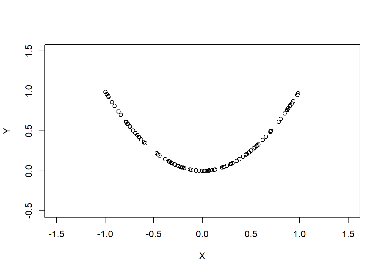
Clearly the relationship between the two random variables is not linear, thus covariance alone would not be a good method to measure the strength of relationship between the two random variables.
The strength of linear relationship between two random variables is hard to determine by solely looking at the covariance because the value depends on how the random variables are scaled. Hence the covariance is often normalized into Pearson correlation coefficient (\(\rho\)), which ranges from -1 to 1, so that it is easier to interpret.
The definition of correlation coefficient is given by: \[\rho_{_{XY}} = \dfrac{Cov[X,Y]}{Sd[X]Sd[Y]} = \dfrac{\sigma_{_{XY}}}{\sigma_{_X}\sigma_{_Y}}\] where \(Sd\) is standard deviation. This is easier to interpret than covariance because it is scaled down to in between -1 and 1. Closer absolute value to 1 means that the linear relationship is stronger.
Properties of covariance
\(Cov[X, a] = 0\)
where a is a constant. In words covariance between a random variable and a constant is 0.
\(Cov[X,X] = Var[X]\)
Covariance of a random variable with itself is a variance.
\(Cov[X,Y] = Cov[Y,X]\)
Covariance of two random variables is the same when the order is flipped. This property leads to the variance-covariance matrix being symmetric
\(Cov[aX,bY] = abCov[X,Y]\)
This property tells me that covariance multiplicately scales corresponding to the changes in the random variables X and Y. This is due to linearity of expectation. The coefficient for each random variable can be pulled out individually because covariance is an expected value of the product of each random variables. Different scaling doesn’t change the strength of relationship, even though higher covariance deceptively indicates so (I could be the only person that had this misconception).
N <- 1000
mu_x <- 5; mu_y <- 5
var_x <- 1; var_y <- 1
cov_xy <- 0.7

bivnorm <- mvrnorm(n = N, mu = c(mu_x, mu_y), Sigma = matrix(c(var_x, cov_xy, cov_xy, var_y), nrow = 2, byrow = TRUE))
par(mfrow = c(1, 2))
plot(bivnorm[,1], bivnorm[,2], xlim = c(1, 9), ylim = c(1, 9), xlab = 'X', ylab = 'Y')
plot(10*bivnorm[,1], bivnorm[,2], xlim = c(10, 90), ylim = c(1, 9), xlab = '10 * X', ylab = 'Y')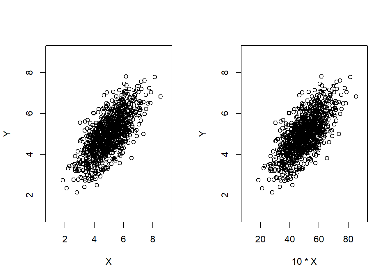
\(Cov[X + a, Y + b] = Cov[X,Y]\)
Like variance, covariance is invariant to locational shifts
\(Cov[aX + bY,cW + dZ] = acCov[X,W] + bcCov[Y,W] + adCov[X,Z] + bdCov[Y,Z]\)
If each coordinate is a linear combination of random variables, then each random variable ‘term’ can be taken out individually. Hence the covariance is equivalent to the summation of the covariance of each ‘pair’ of random variables.
Sample Covariance
Usually population parameters will be unknown and I’ll have to use samples to calculate the covariance. The formula for sample covariance is as follows:
\[Cov[X,Y] = \dfrac{1}{n-1}\sum_{i=i}^{n}(X_i - \bar{X})(Y_i - \bar{Y})\]
This blog translates the calculation of covariance to geometrical sense nicely.
Moving to variance-covariance matrix
Variance-covariance matrix allows us to see covariance of all pairs of components in a random vector. For a random vector \(\textbf{X}\) of length \(N\), the variance-covariance matrix of a random vector X (denote as \(Var(\textbf{X})\), \(Cov(\textbf{X})\), \(\Sigma_\textbf{X}\)) is an \(N \times N\) matrix whose \(i^{th}\) row and \(j^{th}\) is a covariance between \(X_i\) and \(X_j\).
\(\textbf{X} = \begin{pmatrix} X_1 \\ \vdots \\ X_N \end{pmatrix}\)
\(\Sigma_\textbf{X} = \begin{pmatrix} \sigma_{11} & \sigma_{12} & \cdots & \sigma_{1N} \\ \sigma_{21} & \sigma_{22} & \cdots & \sigma_{2N} \\ \vdots & \vdots & \ddots & \vdots \\ \sigma_{N1} & \sigma_{N2} & \cdots & \sigma_{NN} \end{pmatrix}\)
Applying definition of covariance, the \(i^{th}\) row and \(j^{th}\) column is \(\Sigma_{ij} = E\big[(X_i-E[X_i])(X_j-E[X_j])\big]\).
The following are some properties of \(\text{ } \Sigma\) :
The \(i^{th}\) diagonal entry is a variance of an \(i^{th}\) random varible. f \(\Sigma_\textbf{X}\) is a symmetric matrix due to the third property of covariance listed above.
\(\Sigma_\textbf{X}\) is positive semi-definite. In other words, for \(\text{ } \textbf{v} \in \mathbb{R}^N\), \[\textbf{v}^T \Sigma_\textbf{X} \textbf{v} \geq 0\] I’ll provide a simple proof as practice:
\[\textbf{v}^T \Sigma_\textbf{X} \textbf{v} = \textbf{v}^TE\big[(\textbf{X}-E[\textbf{X}])(\textbf{X}-E[\textbf{X}])^T\big]\textbf{v} \] \[= E\big[\textbf{v}^T(\textbf{X}-E[\textbf{X}])(\textbf{X}-E[\textbf{X}])^T\textbf{v}\big] \] \[= E\big[\textbf{v}^T (\textbf{X}-E[\textbf{X}])(\textbf{v}^T(\textbf{X}-E[\textbf{X}]))^T\big] \] \[= E\big[ \big( \textbf{v}^T(\textbf{X}-E[\textbf{X}]) \big)^2 \big] \geq 0 \text{, } \forall \text{ } \textbf{v} \in \mathbb{R}^N\] Note: In the case that \(\exists \text{ } \textbf{v} \in \mathbb{R}^N \text{ s.t. } \textbf{v}^T\Sigma\vec{v} = 0\), there is a component in a random vector \(X\) that can be expressed through linear combination of other components
\(\Sigma_{A\textbf{X}+b} = A\Sigma_\textbf{X}A^T\)
Correlation matrix, (denote as \(\vec{\rho}\)) whose \(i^{th}\) row and \(j^{th}\) column expresses the correlation coefficient between the respective random variables, can be obtained from the variance-covariance matrix.
We know that \(\vec{\rho}_{ij} = \dfrac{Cov(X_i, X_j)}{\sqrt{Var(X_i)Var(X_j)}}\) and the diagnonal entries of \(\text{ } \Sigma \text{ }\) are variances. Hence, \(\vec{\rho} = \big(diag(\Sigma)\big)^{-\frac{1}{2}} \Sigma \big(diag(\Sigma)\big)^{-\frac{1}{2}}\), where \(diag(\Sigma)\) is a diagonal matrix whose diagonal entries are diagonal entries of \(\Sigma\) and other entries 0.
Calculating variance-covariance matrix from a sample
Suppose we have a set of data whose \(\text{ }N\text{ }\)observations are each row and \(\text{ }p\text{ }\) features (variables) are each column. Denote the data by \(\text{ }D\). To calculate for variance-covariance matrix, the values first need to be centered around their mean, then multiplied and summed accordingly.
Let \(\textbf{D}_c\) be data whose values are centered around their mean. Then variance-covariance matrix \(V\) is:
\(V = \dfrac{1}{N-1} \textbf{D}^T_c\textbf{D}_c\)
Example using attitude dataset:
summary(attitude)## rating complaints privileges learning raises
## Min. :40.00 Min. :37.0 Min. :30.00 Min. :34.00 Min. :43.00
## 1st Qu.:58.75 1st Qu.:58.5 1st Qu.:45.00 1st Qu.:47.00 1st Qu.:58.25
## Median :65.50 Median :65.0 Median :51.50 Median :56.50 Median :63.50
## Mean :64.63 Mean :66.6 Mean :53.13 Mean :56.37 Mean :64.63
## 3rd Qu.:71.75 3rd Qu.:77.0 3rd Qu.:62.50 3rd Qu.:66.75 3rd Qu.:71.00
## Max. :85.00 Max. :90.0 Max. :83.00 Max. :75.00 Max. :88.00
## critical advance
## Min. :49.00 Min. :25.00
## 1st Qu.:69.25 1st Qu.:35.00
## Median :77.50 Median :41.00
## Mean :74.77 Mean :42.93
## 3rd Qu.:80.00 3rd Qu.:47.75
## Max. :92.00 Max. :72.00att_c <- sapply(attitude, function(x){x-mean(x)})
cov_att_manual <- 1/(nrow(att_c) - 1) * (t(att_c) %*% att_c)
cov_att <- cov(attitude)
print(cov_att)## rating complaints privileges learning raises critical
## rating 148.17126 133.77931 63.46437 89.10460 74.68851 18.84253
## complaints 133.77931 177.28276 90.95172 93.25517 92.64138 24.73103
## privileges 63.46437 90.95172 149.70575 70.84598 56.67126 17.82529
## learning 89.10460 93.25517 70.84598 137.75747 78.13908 13.46782
## raises 74.68851 92.64138 56.67126 78.13908 108.10230 38.77356
## critical 18.84253 24.73103 17.82529 13.46782 38.77356 97.90920
## advance 19.42299 30.76552 43.21609 64.19770 61.42299 28.84598
## advance
## rating 19.42299
## complaints 30.76552
## privileges 43.21609
## learning 64.19770
## raises 61.42299
## critical 28.84598
## advance 105.85747print(all.equal(cov_att_manual, cov_att))## [1] TRUEAlthough there will almost never be an occasion where I have to calculate the covariance matrix or even other statistics by hand, I thought it would be a good way to practice with matrices and to keep myself aware of the mathematical end of statistics.
There is also another type of covariance matrix called cross-covariance matrix for two random vectors, but I will not go beyond writing the definition.
\[cov(\textbf{X},\textbf{Y}) = E\big[(\textbf{X}-E[\textbf{X}])(\textbf{Y}-E[\textbf{Y}])\big]\]
There is a lot more to covariance and variance-covariance matrix, but this should be enough to found a solid ground for understanding covariance.