Load all the datasets that I’ve saved from the previous benchmarks
set.seed(12345)

library(microbenchmark)
library(tidyverse)
library(knitr)
library(kableExtra)

load("2019-03-01-sorting-comparison/sort_comparisons")
Blowing off the Dust
I see that in my environment, two variables, special_case_sort_time and trend_sort_time are loaded. It’s been a long time since I’ve created these data, so I have an unclear memory as to what these objects are. Usually I use str, class to understand they are. I also make use of head to quickly glance at the data usually if it is a data.frame (glimpse is also a cool function to summarise the data).
class(special_case_sort_time)## [1] "list"str(special_case_sort_time)## List of 3
## $ 10 :List of 5
## ..$ already_sorted :Classes 'microbenchmark' and 'data.frame': 600 obs. of 2 variables:
## .. ..$ expr: Factor w/ 6 levels "bubble_sort",..: 6 5 3 5 5 3 3 1 2 3 ...
## .. ..$ time: num [1:600] 57901 57901 71400 47400 437901 ...
## ..$ sorted_backwards :Classes 'microbenchmark' and 'data.frame': 600 obs. of 2 variables:
## .. ..$ expr: Factor w/ 6 levels "bubble_sort",..: 5 6 3 3 5 3 6 2 3 1 ...
## .. ..$ time: num [1:600] 58101 47601 39600 33000 56701 ...
## ..$ one_off :Classes 'microbenchmark' and 'data.frame': 600 obs. of 2 variables:
## .. ..$ expr: Factor w/ 6 levels "bubble_sort",..: 6 4 1 4 3 4 1 5 2 2 ...
## .. ..$ time: num [1:600] 45401 16700 14201 13000 61800 ...
## ..$ extreme_out_of_place_low :Classes 'microbenchmark' and 'data.frame': 600 obs. of 2 variables:
## .. ..$ expr: Factor w/ 6 levels "bubble_sort",..: 2 3 2 1 4 1 1 1 6 6 ...
## .. ..$ time: num [1:600] 9401 46001 5700 9501 67101 ...
## ..$ extreme_out_of_place_high:Classes 'microbenchmark' and 'data.frame': 600 obs. of 2 variables:
## .. ..$ expr: Factor w/ 6 levels "bubble_sort",..: 6 2 2 1 3 6 5 4 1 2 ...
## .. ..$ time: num [1:600] 49201 9502 6201 17902 55601 ...
## $ 100 :List of 5
## ..$ already_sorted :Classes 'microbenchmark' and 'data.frame': 600 obs. of 2 variables:
## .. ..$ expr: Factor w/ 6 levels "bubble_sort",..: 5 5 6 1 5 2 5 4 1 5 ...
## .. ..$ time: num [1:600] 569901 446700 299702 19401 451901 ...
## ..$ sorted_backwards :Classes 'microbenchmark' and 'data.frame': 600 obs. of 2 variables:
## .. ..$ expr: Factor w/ 6 levels "bubble_sort",..: 5 6 1 2 3 3 6 4 3 4 ...
## .. ..$ time: num [1:600] 481101 370900 1177601 865301 401801 ...
## ..$ one_off :Classes 'microbenchmark' and 'data.frame': 600 obs. of 2 variables:
## .. ..$ expr: Factor w/ 6 levels "bubble_sort",..: 1 2 1 6 6 4 1 3 5 4 ...
## .. ..$ time: num [1:600] 308601 19101 519901 289400 272701 ...
## ..$ extreme_out_of_place_low :Classes 'microbenchmark' and 'data.frame': 600 obs. of 2 variables:
## .. ..$ expr: Factor w/ 6 levels "bubble_sort",..: 1 1 1 3 5 6 1 6 1 4 ...
## .. ..$ time: num [1:600] 44501 38501 41300 459900 471901 ...
## ..$ extreme_out_of_place_high:Classes 'microbenchmark' and 'data.frame': 600 obs. of 2 variables:
## .. ..$ expr: Factor w/ 6 levels "bubble_sort",..: 1 1 2 4 1 5 6 3 3 5 ...
## .. ..$ time: num [1:600] 641501 564401 36502 328301 640101 ...
## $ 1000:List of 5
## ..$ already_sorted :Classes 'microbenchmark' and 'data.frame': 600 obs. of 2 variables:
## .. ..$ expr: Factor w/ 6 levels "bubble_sort",..: 6 2 2 4 2 5 2 6 3 2 ...
## .. ..$ time: num [1:600] 2976501 138901 133901 2159601 138200 ...
## ..$ sorted_backwards :Classes 'microbenchmark' and 'data.frame': 600 obs. of 2 variables:
## .. ..$ expr: Factor w/ 6 levels "bubble_sort",..: 6 6 5 3 6 1 4 2 1 3 ...
## .. ..$ time: num [1:600] 16195401 15706301 7184600 35753601 14458901 ...
## ..$ one_off :Classes 'microbenchmark' and 'data.frame': 600 obs. of 2 variables:
## .. ..$ expr: Factor w/ 6 levels "bubble_sort",..: 6 5 1 1 4 6 5 2 1 4 ...
## .. ..$ time: num [1:600] 3164001 5819700 30979201 56965500 2836000 ...
## ..$ extreme_out_of_place_low :Classes 'microbenchmark' and 'data.frame': 600 obs. of 2 variables:
## .. ..$ expr: Factor w/ 6 levels "bubble_sort",..: 6 3 4 4 3 4 3 1 4 2 ...
## .. ..$ time: num [1:600] 29224901 34690601 2924302 3018901 34510000 ...
## ..$ extreme_out_of_place_high:Classes 'microbenchmark' and 'data.frame': 600 obs. of 2 variables:
## .. ..$ expr: Factor w/ 6 levels "bubble_sort",..: 2 5 4 3 1 4 2 3 5 1 ...
## .. ..$ time: num [1:600] 299802 5845901 2820600 35814002 59596400 ...special_case_sort_time is a list with three elements 10, 100, and 1000. Each is a list containg microbenchmark objects for each special cases.
Attempt #1 at Visualization
For a microbenchmark object, a boxplot method is available to allow us to easily compare different algorithms. autoplot is also available, but I opted with the boxplot. They are essentially the same thing except that autoplot shows the distribution of the data more clearly, which can be done with boxplot by adding another layer of jitter plot.
With the built-in boxplot.microbenchmark, I can visualize the performance of each algorithm.
boxplot(
  special_case_sort_time$`10`$sorted_backwards,
  cex.axis = 0.75,
  unit = "us",
  main = "Performance on Already Sorted Sequence (Length 10)",
  xlab = "Algorithm"
)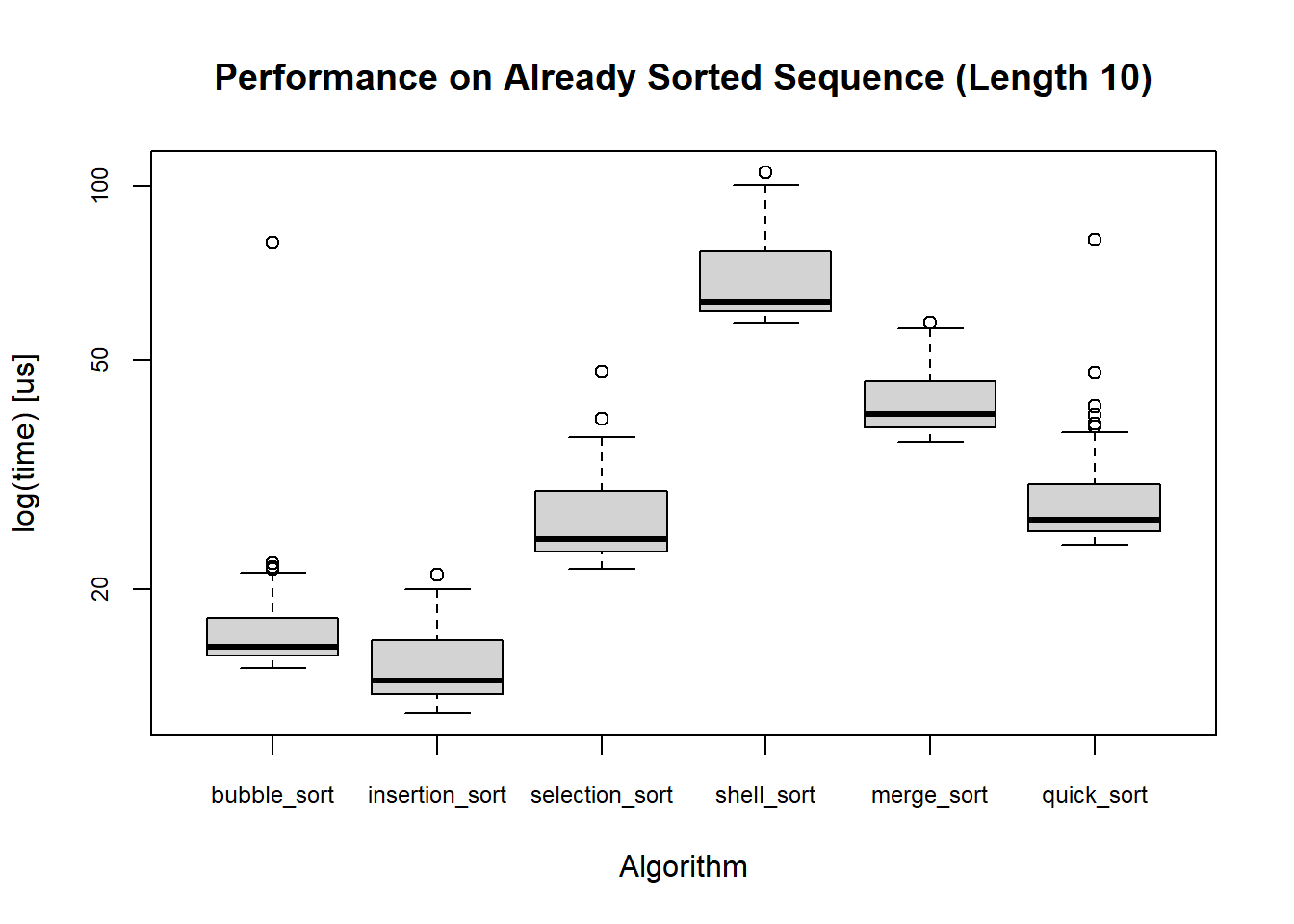
However, using this is limited in a sense that I can only compare algorithms within the same type of sequence. Furthermore, I have contrived sequences with 5 special cases and 6 trends, each of which has 3 lengths. Plotting for all these cases requires repetetive copying and pasting of the code 33 times, which could bore not only the creator of these plots (me) and the reader. Plus, it would be hard to compare across the plots. To give myself more freedom to plot these boxes, I will first make some changes in how the data is stored.
Data Modification
I want my final data.frame to have four columns: expr, time, case, N.
expr: name of the sorting algorithmtime: time in nanosecondscase: name of the special case or trendN: length of the sequence
Since there are two objects which are lists of microbenchmark data (actually a list of lists of microbenchmark data), I created a function to modify both objects into the data.frame, and then combine them.
I wont get into the nitty-gritty of clean_sorting_microbench function, but I’ll provide a quick summary of the function.
- each step is divided by a piping operator,
%>%, available from the packagedplyr - first step (
lapply) involves changing eachmicrobenchmarkto adata.frame, adding a new columncaseto store the name of the cases/trends, and then combine all the cases within each number of sequence lengths - second step (
mapply) adds a new columnNto store the length of sequence. - third step (
do.call) combines alldata.framefrom each sequences lengths.
Of course, this complication can be avoided using for loops, but I like to make use of vectorized nature in R as well as avoid having to keep track of all the variables for each step. Also, piping these allows me to write the function in logical steps.
clean_sorting_microbench <- function(mcb.list) {
  mcb.list %>%
  # for each case in microbench data, swith to data.frame & append a new column "case"
  lapply(
    # for each "length" element, bind all the cases data.frame
    function(x) {
      do.call(
        function(...) rbind(..., make.row.names = FALSE, stringsAsFactors = FALSE),
        mapply(
          # add "case" column
          function(mb, case) cbind(as.data.frame(mb), "case" = case),
          mb = x,
          case = names(x),
          SIMPLIFY = FALSE
        )
      )
    }
  ) %>%
  # add "N" column
  mapply(
    function(a,b) cbind(a, "N" = b),
    a = .,
    b = names(.),
    SIMPLIFY = FALSE
  ) %>%
  # bind all data.frame from separate lengths
  do.call(
    what = function(...) rbind(..., make.row.names = FALSE, stringsAsFactors = FALSE),
    .
  )
}
mydf <- rbind(
clean_sorting_microbench(special_case_sort_time),
clean_sorting_microbench(trend_sort_time)
)
head(mydf)## expr time case N
## 1 quick_sort 57901 already_sorted 10
## 2 merge_sort 57901 already_sorted 10
## 3 selection_sort 71400 already_sorted 10
## 4 merge_sort 47400 already_sorted 10
## 5 merge_sort 437901 already_sorted 10
## 6 selection_sort 48202 already_sorted 10Count Number of Rows
N = 10
| bubble_sort | insertion_sort | selection_sort | shell_sort | merge_sort | quick_sort | |
|---|---|---|---|---|---|---|
| already_sorted | 100 | 100 | 100 | 100 | 100 | 100 |
| extreme_out_of_place_high | 100 | 100 | 100 | 100 | 100 | 100 |
| extreme_out_of_place_low | 100 | 100 | 100 | 100 | 100 | 100 |
| flat_trend | 100 | 100 | 100 | 100 | 100 | 100 |
| left_skew_trend | 100 | 100 | 100 | 100 | 100 | 100 |
| one_off | 100 | 100 | 100 | 100 | 100 | 100 |
| quadratic_trend | 100 | 100 | 100 | 100 | 100 | 100 |
| right_skew_trend | 100 | 100 | 100 | 100 | 100 | 100 |
| sine_trend | 100 | 100 | 100 | 100 | 100 | 100 |
| sorted_backwards | 100 | 100 | 100 | 100 | 100 | 100 |
| symmetrical_trend | 100 | 100 | 100 | 100 | 100 | 100 |
N = 100
| bubble_sort | insertion_sort | selection_sort | shell_sort | merge_sort | quick_sort | |
|---|---|---|---|---|---|---|
| already_sorted | 100 | 100 | 100 | 100 | 100 | 100 |
| extreme_out_of_place_high | 100 | 100 | 100 | 100 | 100 | 100 |
| extreme_out_of_place_low | 100 | 100 | 100 | 100 | 100 | 100 |
| flat_trend | 100 | 100 | 100 | 100 | 100 | 100 |
| left_skew_trend | 100 | 100 | 100 | 100 | 100 | 100 |
| one_off | 100 | 100 | 100 | 100 | 100 | 100 |
| quadratic_trend | 100 | 100 | 100 | 100 | 100 | 100 |
| right_skew_trend | 100 | 100 | 100 | 100 | 100 | 100 |
| sine_trend | 100 | 100 | 100 | 100 | 100 | 100 |
| sorted_backwards | 100 | 100 | 100 | 100 | 100 | 100 |
| symmetrical_trend | 100 | 100 | 100 | 100 | 100 | 100 |
N = 1000
| bubble_sort | insertion_sort | selection_sort | shell_sort | merge_sort | quick_sort | |
|---|---|---|---|---|---|---|
| already_sorted | 100 | 100 | 100 | 100 | 100 | 100 |
| extreme_out_of_place_high | 100 | 100 | 100 | 100 | 100 | 100 |
| extreme_out_of_place_low | 100 | 100 | 100 | 100 | 100 | 100 |
| flat_trend | 100 | 100 | 100 | 100 | 100 | 100 |
| left_skew_trend | 100 | 100 | 100 | 100 | 100 | 100 |
| one_off | 100 | 100 | 100 | 100 | 100 | 100 |
| quadratic_trend | 100 | 100 | 100 | 100 | 100 | 100 |
| right_skew_trend | 100 | 100 | 100 | 100 | 100 | 100 |
| sine_trend | 100 | 100 | 100 | 100 | 100 | 100 |
| sorted_backwards | 100 | 100 | 100 | 100 | 100 | 100 |
| symmetrical_trend | 100 | 100 | 100 | 100 | 100 | 100 |
Well, it looks like this was a success. Now off to do some cool visualizations.
Attempt #2 at Visualization
Now that I have a data.frame in a tidy form, I can use ggplot2 package to various graphs.
I first wanted to compare the performance of each algorithm for each case. The following plot allows me to compare the algorithm performance for each case in each lengths.
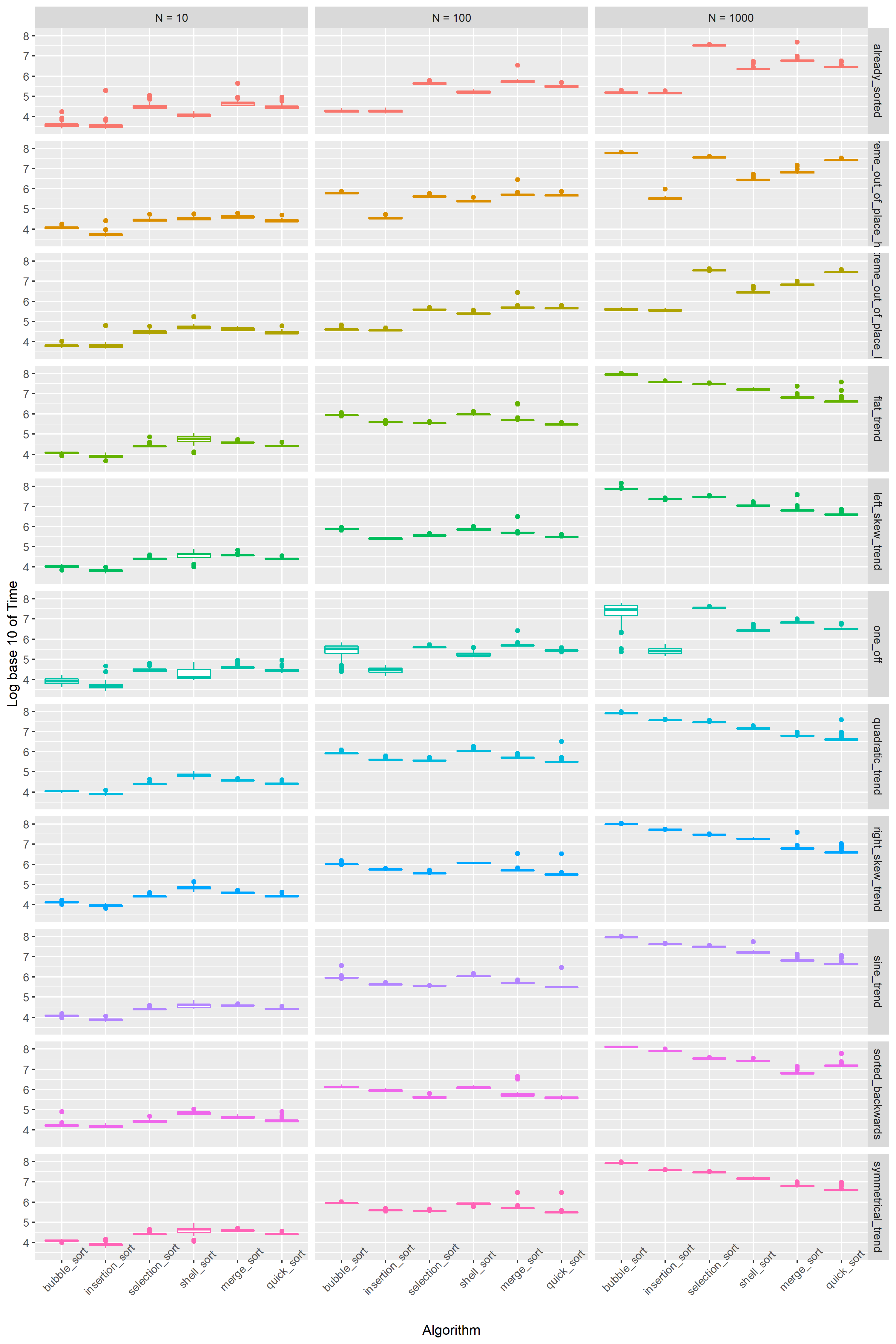
I already see some interesting trends. For each 10 fold increase in the length of the sequence, the average log-time duration for the sorting increases by 1 ~ 2. First off, the sorting can be divided into two kinds of “groups”. First group is comprised of bubble sort, insertion sort, and selection sort. The average time complexity for these algorithms is \(\Theta(n^2)\). In the second group are quick sort, merge sort, and shell sort. The average case for these algorithms is \(\Theta(n log(n))\) (actually for shell sort it’s \(\Theta(n (log(n)^2)\)… explains why this performs closer to \(\Theta(n^2)\) group).
In N = 10, the \(\Theta(n^2)\) group generally outperforms \(\Theta(n log(n))\) group. The two groups have similar performance in N = 100, and \(\Theta(nlog(n))\) group far outperformes the other group in N = 1000.
Some algorithms handle specific cases better than other. We can see that bubble sort consistently does better in all sequence lengths in already_sorted case and extreme_out_of_place_high case. This is expected since the algorithm stops as soon as no swap happens, and bubbles largest values to the top. However the algorithm falls off in all other cases and trends.
We can see that regardless of the trend, when the sequence is large enough, the algorithms of \(\Theta(nlog(n))\) group perform consistently better than others.
What I like about the boxplot is the simplicity as well as the information it gives, especially if many data points are involved. There is a phenomenon that only occurs in one_off case that does not occur in other cases, specifically at N = 100 and N = 1000. While most algorithm’s log-time performance is concentrated around the box / Interquantile Range (IQR), bubble sort’s box shape is much clearer. one_off displaces a single value in a sorted sequence randomly. Because bubble_sort carries the larger value to the top by making a comparison with the next value in line and swapping at every comparison, it is really dependent on when the swap starts happening. My guess is that reliance on the randomness of where the value is displaced caused the variability. I designed the case such that all indices in a sequence has equal chance of being displaced, hence the time to sort the sequence should be uniformly distributed. Since the y-axis of this plot is plotted in log time, a boxplot with some trailing outliers below the lower tail is expected, which is exactly what the box in N = 1000 looks like.
Next plot compares the algorithmic performance in each case. Contrary to the last plot, the cases are “side-by-side”, divided by the algorithm type.
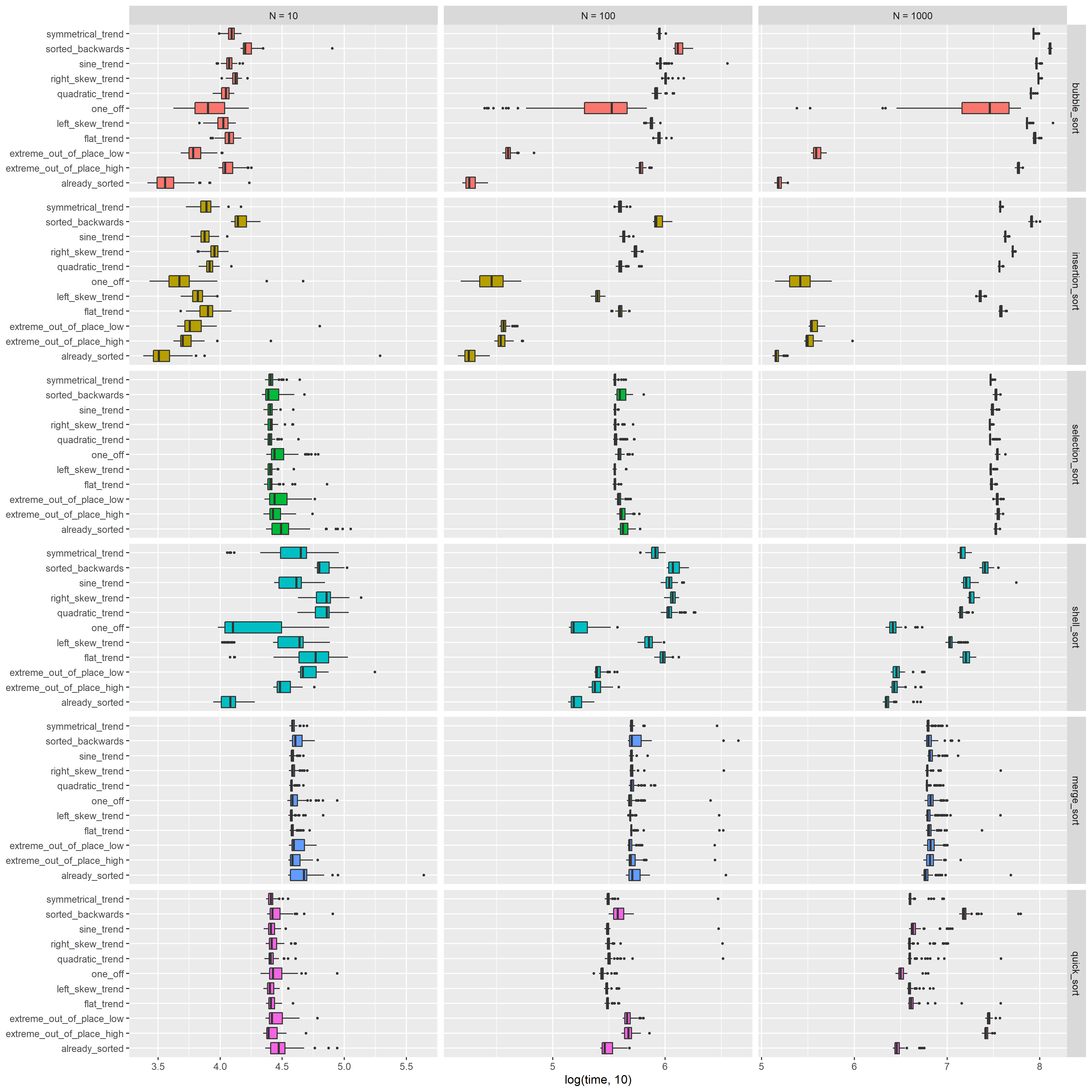
As N gets larger, shell_sort, merge_sort, and quick_sort outperforms the other algorithms, by order of from 10 up to 1000. \(\Theta(n^2)\) group relatively performs well on the special cases than \(\Theta(nlog(n))\) group.
Comparison of Means
For my last trick, maybe comparing the means of each algorithm-case pair could help in visualizing the differences.
Now in here I had two choices for the barplot. The duration increases by factor of ten when the length of sequence also increases by factors of ten. So it’s a good idea to plot y axis on a log scale. I could either calculate the mean first and then log the means, or log-transform the values first and then calculate the log-mean. Turns out, the second method is essentially log of the geometric mean… cool! Anyhow, I think it makes greater sense the use the first approach to compare the means because I’m only really using log to enable visual comparison of the means. Furthermore, interpretation with arithmetic mean in this context after exponentiating seems easier than with geometric mean.
grouped_means <- mydf %>%
  group_by(N, case, expr) %>%
    summarise(mu_time = mean(time)) %>% # arithmatic mean of time
    .[with(., order(N, case,expr)),] %>% # order by N, case, then expr
    ungroup()
## `summarise()` has grouped output by 'N', 'case'. You can override using the `.groups` argument.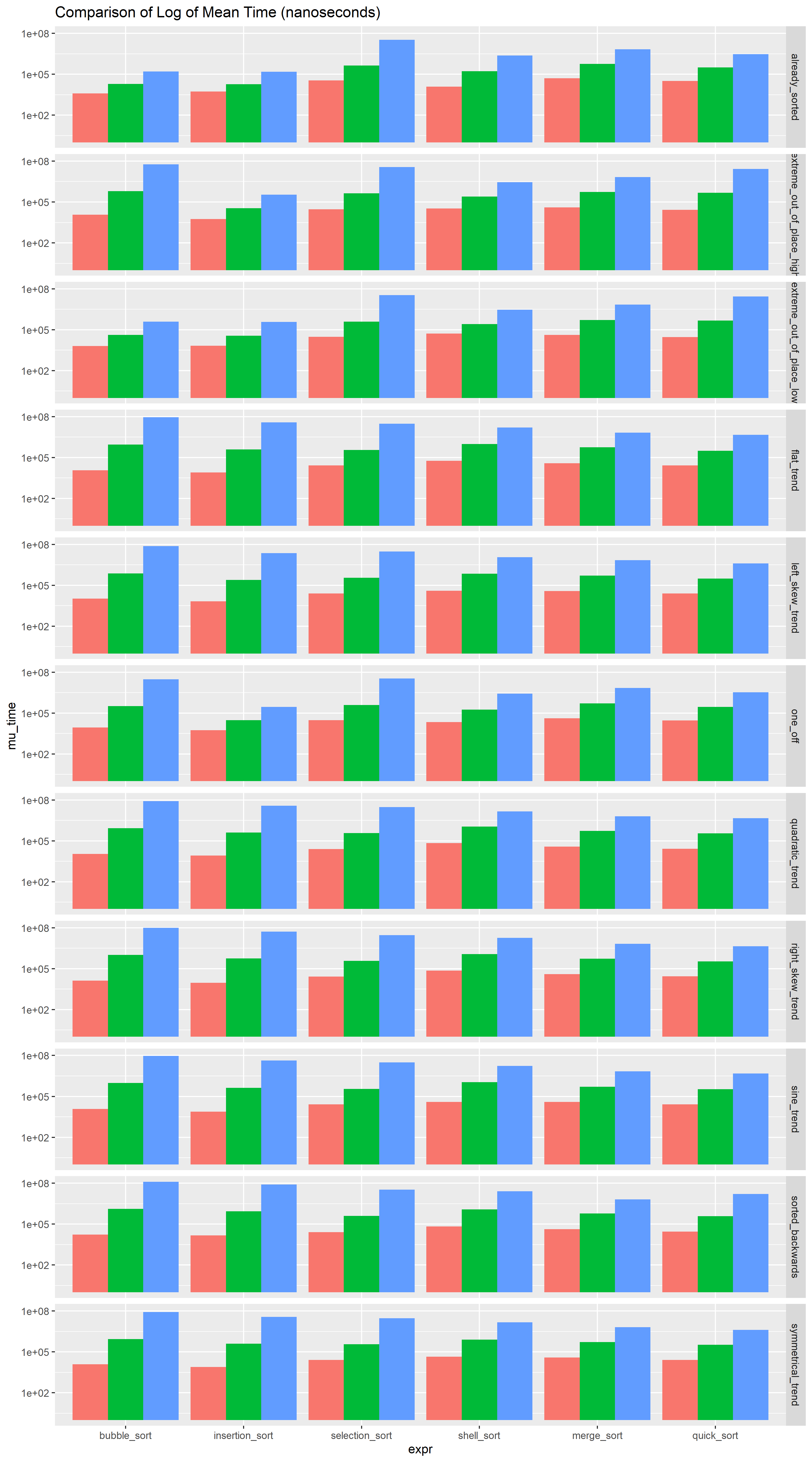
As interesting as this plot really is, it’s honestly hard to see the real differences in changes in duration of the sort. I am curious to see if plotting the differences between the lengths help. The duration grows multiplicatively, which means I’ll be dividing to quantify the jump in the duration when the length of sequence is changed.
grouped_means_10 <-
  dplyr::filter(grouped_means, N == 10) %>%
    dplyr::rename("mu_time_10" = mu_time) %>%
    dplyr::select(-N)
grouped_means_100 <- dplyr::filter(grouped_means, N == 100) %>%
  dplyr::rename("mu_time_100" = mu_time) %>%
    dplyr::select(-N)
grouped_means_1000 <- dplyr::filter(grouped_means, N == 1000) %>%
  dplyr::rename("mu_time_1000" = mu_time) %>%
    dplyr::select(-N)

grouped_means_diff <-
  grouped_means_10 %>%
    full_join(grouped_means_100, by = c("case", "expr")) %>%
    full_join(grouped_means_1000, by = c("case", "expr")) %>%
    mutate(
      diff_10_100 = mu_time_100 / mu_time_10,
      diff_100_1000 = mu_time_1000 / mu_time_100,
      diff_10_1000 = mu_time_1000 / mu_time_10
    ) %>%
    dplyr::select(case, expr, contains("diff")) %>%
    gather(key = "N_compared", value = "time_diff", diff_10_100:diff_10_1000) %>%
  mutate("N_compared" = factor(N_compared, c("diff_10_100", "diff_100_1000", "diff_10_1000")))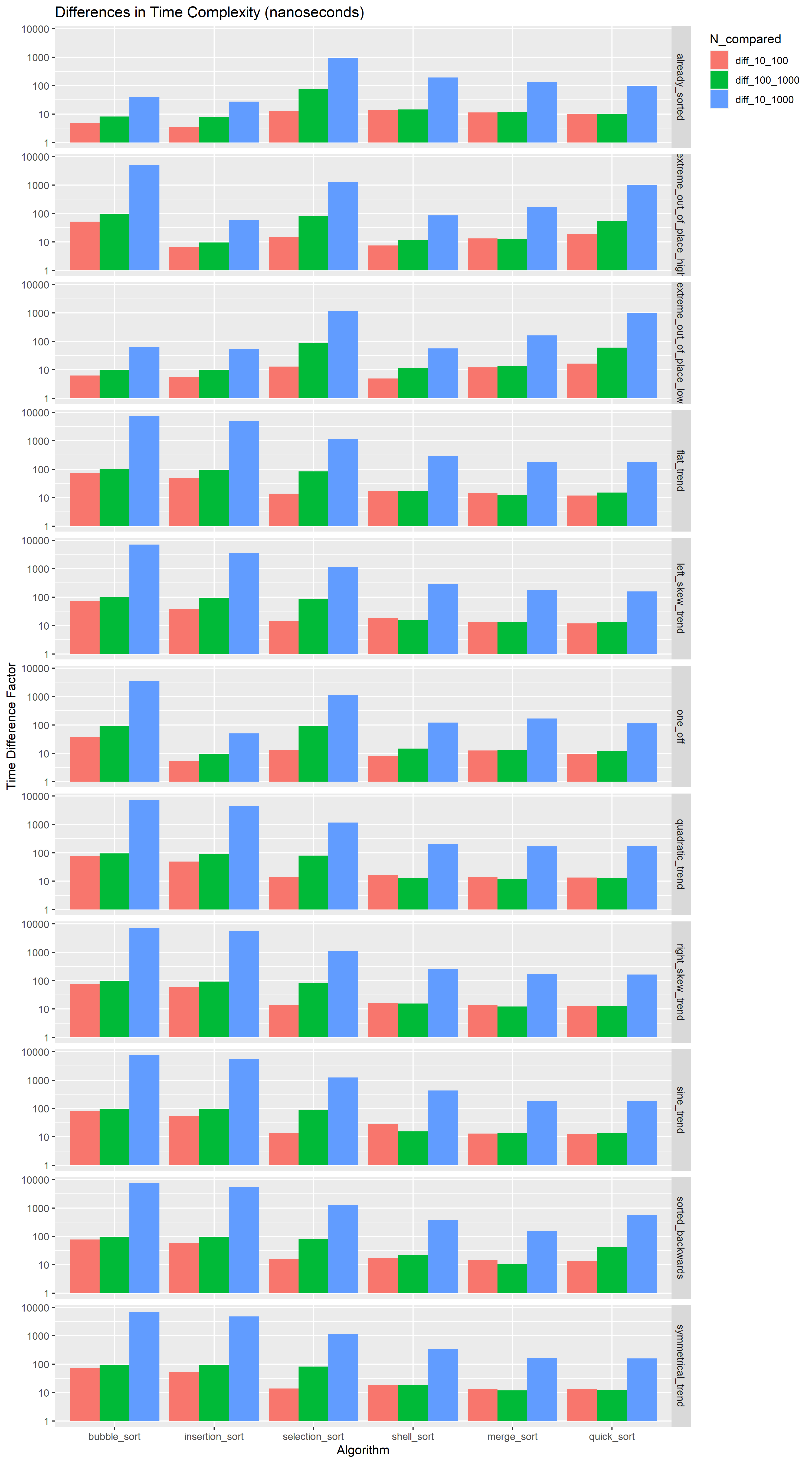
You can actually see here the time difference between varying lengths. Let’s focus on the blue bar, which represents the jump from N = 10 to N = 1000, and on the trends. The duration increases by factors of almost 5000 (the plot is on the log scale) for bubble_sort and insertion_sort. selection_sort scales surprisingly well, comparably so to the other three best performing algorithms. The \(\Theta(n log(n))\) groups scale well. According to the barplot, the time scales almost linearly with the length.
For me, there’s something soothing about looking at plots places side by side for comparison. I can kind of zone out while at the same time trying to figure out the pattern. I hoped I helped the readers realize the versatility of visualization, and the difference in information conveyed, even with the same data, just by making a few changes such as switching up the x-axis and y-axis, changing the grouping variable, or manipulating the numbers.